From Data to Decisions – 历史的进程

课程网站-Chris Mack-The University of Texas at Austin
Youtube-视频合集
 NIST/SEMATECH e-Handbook of Statistical Methods
Six Sigma-Response Surface Modeling
Response Surface Methodology-荧光粉

Data and Measurement

What is Data? (Data = the results of a measurement)

Definition of the thing being measured
Measurement value (number plus units)
Estimate of the uncertainty of each measurement
Experimental context (measurement method + environment)
Context uncertainty (uncertainty of controlled and uncontrolled input parameters)
Measurement model (theory, assumptions and definitions used in making the measurement)
几乎所有的测量都是indirect，我们实际是不是测量我们真正想要的东西，而是测量something else and then we're relating the thing we measure to the thing we want.

The Measurement Model

Virtually all measurements are indirect
— We have a set of theories that relate what is actually being measured to what we want to measure (measurement model)
Ex: Measuring temperature with a thermometer
- - Thermal expansion of mercury (or spirits) turns length measurement into temperature measurement
  - Theory: linear model of liquid thermal expansion
Ex: Measuring temperature with a thermocouple
- - Junction of dissimilar metals turns temperature change into voltage change (Seebeck effect)
  - Theory: polynomial model of voltage versus temperature, coupled with digital (or analog) voltage measurement.

Measurement is not a Passive Act

Measurement can change the thing you are measuring
— Measurement is often not observation without disturbance
Example: SEM measurement
- - Sample charging
  - Physical and chemical changes of sample due to electron bombardment 电子轰击 (carbon deposition, etc.)
  - Effects can be current and voltage dependent

All Measurements are Uncertain

Measurement error exists, but we do not know what it is
- - If we knew the measurement error, we would subtract it out!
  - Unknown errors are called uncertainties
Our goal is to estimate the uncertainty in our measurements
- - Random errors can be estimated using repeated measurements
  - Systematic errors require a sophisticated understanding of the measurement process (and the measurement model)

Measurement Stability

We often make assumptions of spatial and/or temporal stability of measurements.
- - Repeated measurements are taken at different times, locations, conditions, etc.
  - How constant is the sample?
  - How constant is the measurement process?
  - How constant is the measurement context?

Measurement Terms

【Metrology】(计量学/ 量测学/ 量衡学): the science of measurement.
【Measurand】(被测物): the thing being measured.
【True Value】: the unknown (and unknowable) thing we wish to estimate.
【Error】: true value – measured value.
【Measurement Uncertainty】: an estimate of the dispersion of measurement values around the true value.

Uncertainty Components

【Systematic errors】
- - Produce a bias in the measurement result.
  - We look for and try to correct for all systematic errors, but we are never totally successful.
  - We try to put an upper limit on how big we expect systematic errors could be.
【Random errors】
— Can be evaluated statistically, through repeated measurements.

Other Measurement Terms

【Accuracy】(准确度): the same as error, it can never be known, but is estimated as the maximum systematic error that might reasonably exist
【Precision】(精密度): the standard deviation of repeated measurements (random error component). 精密仪器Precision Instrument
- - 【Repeatability】: standard deviation of repeated measurements under conditions as nearly identical as possible. 侧重于自己在原来的仪器(样品)上重复试验。
  - 【Reproducibility】: standard deviation of repeated measurements under conditions that vary in a typical way (different operators, instruments, days). 侧重比如自己观察到的实验现象，别人是否能在他自己的仪器上观察到。
对于上面右侧的图，Wiki给的说明是Accuracy is the proximity of measurement results to the accepted value; precision is the degree to which repeated (or reproducible) measurements under unchanged conditions show the same results.

Measurement Model Example

How wide is this feature?
Most critical dimension measurement tools use a trapezoidal (梯形的) feature model
- - What criterion should be used to best fit a trapezoid to this complicated shape?
  - Accuracy of the width measurement is a strong function of the appropriateness of the feature model (not a good fit means not a good measurement)
The measurement model of an SEM = the feature model + a model for how electrons interact with the sample

Data Example

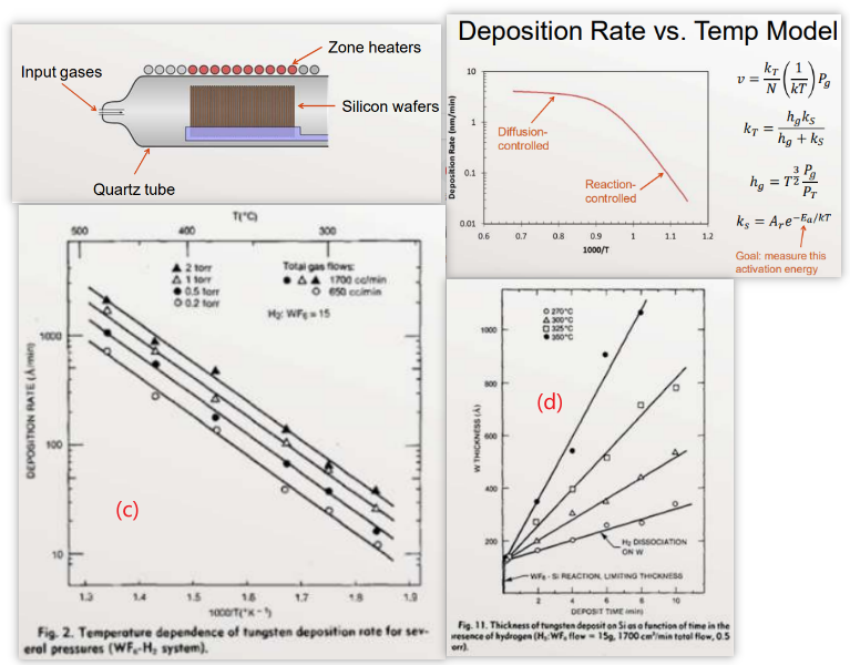
Chemical vapor deposition (CVD) is used to deposit a tungsten film on a silicon wafer

图(c)

There is no mention of deposition rate measurement error
"The temperature was controlled to within ± 2ºC of the desired value within the deposition zone."
The context of the experiment is well described
There was no mention of context uncertainty (ex: pressure, flow rates)
"From the Arrhenius plots an activation energy, E_a, of 0.71 eV/atom (69,000 J/mol) was calculated."实际上不同的线拟合的结果应该有差异。

图(d)

Deposition rate is the slope of these lines (presumably determined by ordinary least squares regression)
What is the uncertainty (standard error) in the slopes?
What assumptions are being made here? Can the assumptions be tested? (指的是沉积厚度和沉积时间的线性关系)

Process Modeling

Introduction

Introduction to Process Modeling-NIST
Process modeling is the concise description of the total variation in one quantity $y$ (called the response variable) by partitioning (分割，分开) it into
- - - A deterministic component (确定性的成分) given by a mathematical function of one or more other quantities, $x_{1}, x_{2}, \ldots$ and possibly unknown coefficients $\beta_{0}, \beta_{1}, \ldots$
    - A random component $\varepsilon$ that follows a particular probability distribution $$ y=f(\boldsymbol{x}, \boldsymbol{\beta})+\varepsilon \quad \boldsymbol{x}=\left(x_{1}, x_{2}, \ldots\right) ; \boldsymbol{\beta}=\left(\beta_{0}, \beta_{1}, \ldots\right) $$
Generally, we require $\mathrm{E}[\varepsilon]=0$.
— Thus $f(\boldsymbol{x}, \boldsymbol{\beta})$ describes the average response, $\mathrm{E}[y]$, if the experiment is repeated many times, not the actual response for a given trial
Our three tasks in modeling:
- - Find the equation from $f(\boldsymbol{x}, \boldsymbol{\beta})$ that meets our goals
  - Find the values of the coefficients $\beta$ that are "best" in some sense
  - Characterize the nature of $\varepsilon$ (distribution of errors)
The 【perfect model】 has
- - The correct set of input variables $x_{1}, x_{2}, \ldots$
  - The correct model form $f(\boldsymbol{x}, \boldsymbol{\beta})$
  - The correct values for the coefficients $\beta_{0}, \beta_{1}, \ldots$
  - The correct probability distribution for $\varepsilon$, including parameters such as its standard deviation $\sigma$
Picking the right model (form and predictor variables) is called 【modeling building】
Finding the best estimate of the parameter values and the properties of the random variable $\varepsilon$ is called 【regression】

Model Generalizability

$y=f(\boldsymbol{x}, \boldsymbol{\beta})+\varepsilon$

The three aspects of our model (equation, coefficients, and errors) can have different levels of generalizability
— We often want to know the levels of generalizability
Example: model of thermal stress on polymer
- - The equation form applies to all materials (under certain conditions)
  - The parameters change for different materials
  - The errors are a function of measurement and experimental methods, independent of materials

Some Terminology

$y=$ response variable, response, dependent variable
$x=$ predictor variable, explanatory variable, independent variable, predictor, regressor
Our "model" is both the function $f(\boldsymbol{x}, \boldsymbol{\beta})$ and the assumed distribution of $\varepsilon$

Regression

Regression involves three things:
- - Data (a response variable as a function of one or more predictor variables)
  - Model (fixed form and predictor variables, but with unknown parameters)
  - Method (a statistical regression technique appropriate for the model and the data to find the “best” values of the model parameters)
High quality regression requires high quality in all three items

The Model

Statistical Relationship: $y_{i}=f\left(x_{i}, \beta\right)+\varepsilon_{i}=\hat{y}_{i}+\varepsilon_{i}$
Functional Relationship: $\hat{y}=f(x, \beta)$ or $E[Y \mid X]=f(X, \beta)$
$X, Y=$ random variables (probability terminology)
$\hat{y}=$ predicted (mean) response
$y_{i}=$ measured response for $\mathrm{i}^{\text {th }}$ data point
$x_{i}=$ value of explanatory variable for $\mathrm{ith}^{\text {th }}$ data point
$X, Y=$ random variables (probability terminology)
$\hat{y}=$ predicted (mean) response
$Y_{i}=$ measured response for $\mathrm{i}^{\text {th }}$ data point
$X_{i}=$ value of 【explanatory variable】 (解释变量，其实就是自变量) for $\mathrm{i}^{\text {th }}$ data point
$\beta_{k}=$ true model parameters (can never be known)
$b_{k}=$ best fit model parameters for this data set (sample); our estimate for $\beta_{k}$.
$\varepsilon_{i}=$ true value of $\mathrm{i}^{\text {th }}$ residual (from true model, not known)
$e_{i}=$ actual ith residual for the current model

Example Model

Straight line model:$$ \begin{aligned} &f(x, \beta)=\beta_{0}+\beta_{1} x \\ &\hat{y}_{i}=\beta_{0}+\beta_{1} x_{i} \\ &y_{i}=\beta_{0}+\beta_{1} x_{i}+\varepsilon_{i} \end{aligned} $$
Regression produces the "best" estimate of the model given the data $\left(x_{i}, y_{i}\right)$ :$$ y_{i}=b_{0}+b_{1} x_{i}+e_{i} $$

Models for Linear Regression

We use linear regression for 【linear parameter models】: $\hat{y}$ is directly proportional to each unknown model coefficient
- - $\hat{y}=\sum_{k} \beta_{k} f_{k}(x)$ for bivariate data (双变量数据)
  - Example: $\hat{y}=\beta_{0}+\beta_{1} x+\beta_{2} x^{2}+\beta_{3} \ln (x)$
Multivariate data: two or more explanatory variables (we'll call them $x_{1}, x_{2}$, etc.)

Nonlinear Regression

We call our regression nonlinear if it is nonlinear in the coefficients
- - Linear regression: $\hat{y}=\beta_{0}+\beta_{1} \ln (x)+\beta_{2} x^{3}$
  - Nonlinear regression: $\hat{y}=\beta_{0} e^{\beta_{1} x}$
  - (非)线性回归，其实就是说应变量能不能表示为多个待定系数的线性组合，其中每一个待定系数都和一个含有自变量$x $的表达式相乘。比如函数$f(x, \boldsymbol{\beta})=\displaystyle\frac{\beta_{1} x}{\beta_{2}+x}$是非线性的，因为它不能表示为两个$\beta$的线性组合。非线性函数的其他示例包括指数函数，对数函数，三角函数，幂函数，高斯函数和洛伦兹曲线。某些函数（如指数函数或对数函数）可以进行转换，以使它们是线性的。如此转换，可以执行标准线性回归，但必须谨慎应用。
Linear regression is relatively easy
— Numerically stable with unique solution given a reasonable definition of "best" fit
Nonlinear regression is relatively hard

Regression Review

Vocabulary

Experiment — explanatory variables are manipulated (controlled), all other inputs are held constant, and the response variable is measured
但是对于observation来说，我们测试inputs和outputs，也不控制inputs
Model — a mathematical function that approximates the data and is useful for making predictions
Regression — a method of finding the best fit of a model to a given set of data through the adjustment of model parameters (coefficients)
— What do we mean by “best fit”?
Residual: $\varepsilon_{i}=y_{i}-f\left(\boldsymbol{x}_{\boldsymbol{i}}, \boldsymbol{\beta}\right), e_{i}=y_{i}-f\left(\boldsymbol{x}_{\boldsymbol{i}}, \boldsymbol{b}\right)$
residual可能是error in the mdel and/or model；这里的$\boldsymbol{\beta}$是model理论上参数，我们无法知道，但是可以用$\boldsymbol{b}$去估计。
A "good" model has small residuals
- - Small mean, $|\bar{\varepsilon}|$
  - Small variance (方差), $\sigma_{\varepsilon}^{2}$
Much of our model and regression checking will involve studying and plotting residuals
— Plot $e_{i} v s . \hat{y}_{i}$ (works for multiple regression)

What Do We Mean by “Best Fit”?

First, assume $\varepsilon$ is a random variable that does not depend on $x$
- - There are no systematic errors
  - The model is perfect
Desired properties of a "best fit" estimator
- - Unbiased, $\sum \varepsilon_{i}=\sum e_{i}=0\left(\right.$ and $\left.E\left[b_{k}\right]=\beta_{k}\right)$(其实就是实验次数无穷大时的收敛值)
  - Efficient, minimum variance $\sigma_{e}^{2}\left(\right.$ and $\left.\operatorname{var}\left(b_{k}\right)\right)$
  - Maximum likelihood (for an assumed pdf of $\varepsilon$ )
  - Robust (to be discussed later)
    鲁棒性，if I have a or a few bad data point(s), how much does it screw up answer。

Maximum Likelihood Estimation

【Likelihood function】: the probability of getting this exact data set given a known model and model parameters
— To calculate the likelihood function, we need to know the joint probability distribution function (pdf) of $\varepsilon$
【Maximum Likelihood】: what parameter values maximize the likelihood function?
- - Take the partial derivative of the likelihood function (or more commonly the log-likelihood function) with respect to each parameter, set it equal to zero
  - Solve resulting equations simultaneously

MLE Example – straight line

Let $y_{i}=\beta_{0}+\beta_{1} x_{i}+\varepsilon_{i}, \varepsilon_{i} \sim N\left(0, \sigma_{\varepsilon}\right)$, iid
Since each $\varepsilon_{i}$ is independent, the likelihood function for the entire data set is$$ L=\prod_{i=1}^{n} \mathbb{P}\left(y_{i}\right)=\prod_{i=1}^{n} \mathbb{P}\left(\varepsilon_{i}\right) $$
Since the residuals are iid Normal,$$ L=\left(\frac{1}{\sqrt{2 \pi} \sigma_{\varepsilon}}\right)^{n} \exp \left[-\frac{1}{2} \sum_{i=1}^{n} \frac{\varepsilon_{i}^{2}}{\sigma_{\varepsilon}^{2}}\right] $$
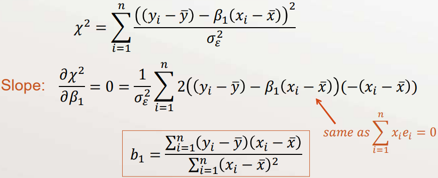
Define chi-square as$$ \chi^{2}=\sum_{i=1}^{n} \frac{\varepsilon_{i}^{2}}{\sigma_{\varepsilon}^{2}} \quad \text { (also called weighted SSE) } $$
Maximizing $L$ is the same as minimizing $\chi^{2}$
Solve these equations simultaneously$$ \frac{\partial \chi^{2}}{\partial \beta_{k}}=0 \text { for all } k \text { (all coefficients) } $$
For our line model, $\varepsilon_{i}=y_{i}-\left(\beta_{0}+\beta_{1} x_{i}\right)$
Substitute our estimate for $\beta_{0}$ into $\chi^{2}$

Assumptions for this MLE

We assumed three things:
- Each residual (and $y_{i}$ ) is independent
- Each residual (and $y_{i}$ ) is identically distributed
- Each $\varepsilon_{i} \sim N\left(0, \sigma_{\varepsilon}\right)$, and thus $y_{i} \sim N\left(\hat{y}, \sigma_{\varepsilon}\right)$
- We call this 【ordinary least squares】 (OLS)
If any of these assumptions are invalid, then our least-squares estimates will not be the maximum likelihood estimates

Properties of our OLS Solution

The parameters are unbiased estimators of the true parameters, with minimum variance compared to all other unbiased estimators (if our assumptions are correct)
$\displaystyle\sum_{i=1}^{n} e_{i}=0$
$\displaystyle\sum_{i=1}^{n} y_{i}=\displaystyle\sum_{i=1}^{n} \hat{y}_{i}$, so that $\bar{y}=\overline{\hat{y}}$
$\displaystyle\sum_{i=1}^{n} \hat{y}_{i} e_{i}=0$
$\displaystyle\sum_{i=1}^{n} x_{i} e_{i}=0$
The best fit line goes through the point $(\bar{x}, \bar{y})$

OLS Matrix Formulation

When we have multivariate data, it is most convenient to formulate the OLS/MLE problem using matrix math

$i=1,2,3, \ldots, n$ data point index
$k=0,1,2, \ldots, p-1$ predictor variable index
$x_{i, k}=i^{t h}$ value for the $k^{t h}$ predictor variable
$y_{i}=i^{t h}$ response data value
$\hat{y}=\beta_{0}+\beta_{1} x_{1}+\beta_{2} x_{2}+\cdots+\beta_{p-1} x_{p-1}$

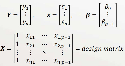
Model in matrix form: $\boldsymbol{Y}=\boldsymbol{X} \boldsymbol{\beta}+\boldsymbol{\varepsilon}$
(each row in $X$ and $\boldsymbol{Y}$ is a "data point")

Sum of square errors$$ S S E=\sum_{i=1}^{n} \varepsilon_{i}^{2}=\boldsymbol{\varepsilon}^{T} \boldsymbol{\varepsilon}=(\boldsymbol{Y}-\boldsymbol{X} \boldsymbol{\beta})^{T}(\boldsymbol{Y}-\boldsymbol{X} \boldsymbol{\beta}) $$

Maximum Likelihood estimate (minimum SSE): $$ \frac{\partial \chi^{2}}{\partial \beta_{k}}=0=\sum_{i=1}^{n} x_{i, k} \varepsilon_{i} \text { giving } \boldsymbol{X}^{\boldsymbol{T}} \boldsymbol{\varepsilon}=\mathbf{0} $$Using the definition of the residual, $ \boldsymbol{X}^{T} \boldsymbol{X} \boldsymbol{\beta}=\boldsymbol{X}^{T} \boldsymbol{Y}$

Minimum SSE occurs when the coefficients are estimated as $$ \begin{gathered} \widehat{\boldsymbol{\beta}}=\left(\boldsymbol{X}^{T} \boldsymbol{X}\right)^{-1} \boldsymbol{X}^{T} \boldsymbol{Y} \\ \widehat{\boldsymbol{Y}}=\boldsymbol{X} \widehat{\boldsymbol{\beta}}=\boldsymbol{X}\left(\boldsymbol{X}^{T} \boldsymbol{X}\right)^{-1} \boldsymbol{X}^{T} \boldsymbol{Y}=\boldsymbol{H} \boldsymbol{Y} \\ \boldsymbol{H}=\boldsymbol{X}\left(\boldsymbol{X}^{T} \boldsymbol{X}\right)^{-1} \boldsymbol{X}^{T}=\text { hat matrix } \\ \boldsymbol{e}=\boldsymbol{Y}-\widehat{\boldsymbol{Y}}=(\boldsymbol{I}-\boldsymbol{H}) \boldsymbol{Y} \end{gathered} $$注意$\boldsymbol{I}$表示的是identity matrix；$\boldsymbol{H}$和$\boldsymbol{I}-\boldsymbol{H}$都是symmetric；common alternate notation: $b_{k}=\hat{\beta}_{k}$

We can use our solution to calculate the covariance matrices:$$ \begin{gathered} \operatorname{cov}(\boldsymbol{e})=s_{e}^{2}(\boldsymbol{I}-\boldsymbol{H}), \quad \operatorname{var}\left(e_{i}\right)=s_{e}^{2}\left(1-h_{i i}\right) \\ \operatorname{cov}\left(e_{i}, e_{j}\right)=-s_{e}^{2} h_{i j} \\ \operatorname{cov}(\widehat{\boldsymbol{Y}})=s_{e}^{2} \boldsymbol{H}, \quad \operatorname{var}\left(\hat{y}_{i}\right)=s_{e}^{2} h_{i i} \\ \operatorname{cov}(\widehat{\boldsymbol{\beta}})=s_{e}^{2}\left(\boldsymbol{X}^{T} \boldsymbol{X}\right)^{-1} \end{gathered} $$其中$s_{e}^{2}$是Variance of the residuals。

MLE Straight-Line Regression

Our model: $E[Y \mid X]=\beta_{0}+\beta_{1} X$$$ \begin{aligned} &\beta_{1}=\frac{\operatorname{cov}(X, Y)}{\operatorname{var}(X)} \\ &\beta_{0}=E[Y]-\beta_{1} E[X] \end{aligned} \quad \rho=\frac{\operatorname{cov}(X, Y)}{\sqrt{\operatorname{var}(X) \operatorname{var}(Y)}} $$
Ordinary least squares (OLS) estimators:$$ b_{1}=\frac{\sum_{i=1}^{n}\left(x_{i}-\bar{x}\right)\left(y_{i}-\bar{y}\right)}{\sum_{i=1}^{n}\left(x_{i}-\bar{x}\right)^{2}} \quad b_{0}=\bar{y}-b_{1} \bar{x} $$

Uncertainty of Fit Parameters

The regression fit is based on a sample of data$$ \text { Population Model: } y_{i}=\beta_{0}+\beta_{1} x_{i}+\varepsilon_{i} $$
To create confidence intervals for $b_{0}, b_{1}$, and $\hat{y}_{i}$, we need to know their sampling distributions
— Given the assumption of $\varepsilon_{i} \sim N\left(0, \sigma_{\varepsilon}^{2}\right)$, the parameter sampling distributions are unbiased and t-distributed (DF = n-2) degrees of freedom)
$$ \begin{gathered} \operatorname{var}\left(b_{1}\right)=\frac{\operatorname{var}(\varepsilon)}{n \operatorname{var}(X)} \quad \operatorname{var}\left(b_{0}\right)=\frac{\operatorname{var}(\varepsilon)}{n}\left(1+\frac{\bar{x}^{2}}{\operatorname{var}(X)}\right) \\ \operatorname{cov}\left(b_{0}, b_{1}\right)=-\bar{x} \operatorname{var}\left(b_{1}\right) \end{gathered} $$
Estimators: (其中$p$表示number of model parameters)$$ \begin{gathered} s_{e}^{2}=\frac{1}{n-p} \sum_{i=1}^{n} e_{i}^{2} \\ s_{b 1}^{2}=\frac{s_{e}^{2}}{(n-1) s_{x}^{2}} \quad s_{b 0}^{2}=\frac{s_{\varepsilon}^{2}}{n}+s_{b 1}^{2} \bar{x}^{2} \end{gathered} $$

Confidence Intervals

The sampling distributions are Student's t with DF = n – 2
- Slope CI: $b_{1} \pm t_{n-2, \alpha} s_{b 1} \quad s_{b 1}^{2}=\displaystyle\frac{s_{\varepsilon}^{2}}{(n-1) s_{x}^{2}}$
- Intercept CI: $b_{0} \pm t_{n-2, \alpha} s_{b 0} \quad s_{b 0}^{2}=\displaystyle\frac{s_{\varepsilon}^{2}}{n}+s_{b 1}^{2} \bar{x}^{2}$
  其中$n$是Critical t-value，$\alpha=$是significance level (e.g., 0.05)

Uncertainty of Predictions

Uncertainty in $\hat{y}_{i}$ comes from the spread of the residuals and from uncertainty in the best fit parameters $b_{1}$ and $b_{0}$$$ \begin{aligned} \operatorname{var}\left(\hat{y}_{i}\right) &=\frac{\operatorname{var}(\varepsilon)}{n}\left(1+\frac{\left(x_{i}-\bar{x}\right)^{2}}{\operatorname{var}(X)}\right) \\ s_{\hat{y}_{i}}^{2} &=\frac{s_{\varepsilon}^{2}}{n}+s_{b 1}^{2}\left(x_{i}-\bar{x}\right)^{2} \end{aligned} $$
Uncertainty in a predicted new measurement $\hat{y}_{\text {new }}$ adds additional uncertainty of a single measurement$$ s_{\hat{y}_{n e w}}^{2}=s_{\hat{y}_{i}}^{2}+s_{\varepsilon}^{2} $$

Uncertainty of Correlation Coefficient

$$ \rho=\frac{\operatorname{cov}(X, Y)}{\sqrt{\operatorname{var}(X) \operatorname{var}(Y)}} \quad r=\frac{1}{n-1} \sum_{i=1}^{n}\left(\frac{x_{i}-\bar{x}}{s_{x}}\right)\left(\frac{y_{i}-\bar{y}}{s_{y}}\right) $$

The sampling distribution for $r$ is about Student's t (D F=n-2) only for $\rho=0$. For this case$$ S_{r}=\frac{s_{\varepsilon}}{\sqrt{n-1} s_{y}} $$
For $\rho \neq 0$, the sampling distribution is complicated
We’ll use the Fisher z-transformation: $$ z=\frac{1}{2} \ln \left(\frac{1+r}{1-r}\right) $$
When $n>25, z$ is about normal with$$ E[z]=\frac{1}{2} \ln \left(\frac{1+\rho}{1-\rho}\right) \quad \operatorname{var}(z)=\frac{1}{n-3} $$

Assumptions in OLS Regression

$\varepsilon$ is a random variable that does not depend on $x$ (i.e., the model is perfect, it properly accounts for the role of $x$ in predicting $y$ )
$\mathrm{E}\left[\varepsilon_{l}\right]=0$ (the population mean of the true residual is zero); this will always be true for a model with an intercept
All $\varepsilon_{i}$ are independent of each other (uncorrelated for the population, but not for a sample)
All $\varepsilon_{j}$ have the same probability density function (pdf), and thus the same variance (called homoscedasticity)
$\varepsilon \sim \mathrm{N}\left(0, \sigma_{\varepsilon}\right)$ (the residuals, and thus the $y_{i}$, are normally distributed)
The values of each $x_{i}$ are known exactly

Checking the Assumptions

Do the assumptions in OLS regression hold?
— Which assumptions can you validate?
— If an assumption is violated, how far off is it?
If one or more assumptions do not hold, does the observed violation invalidate the statistical procedure used?
— If so, what next?

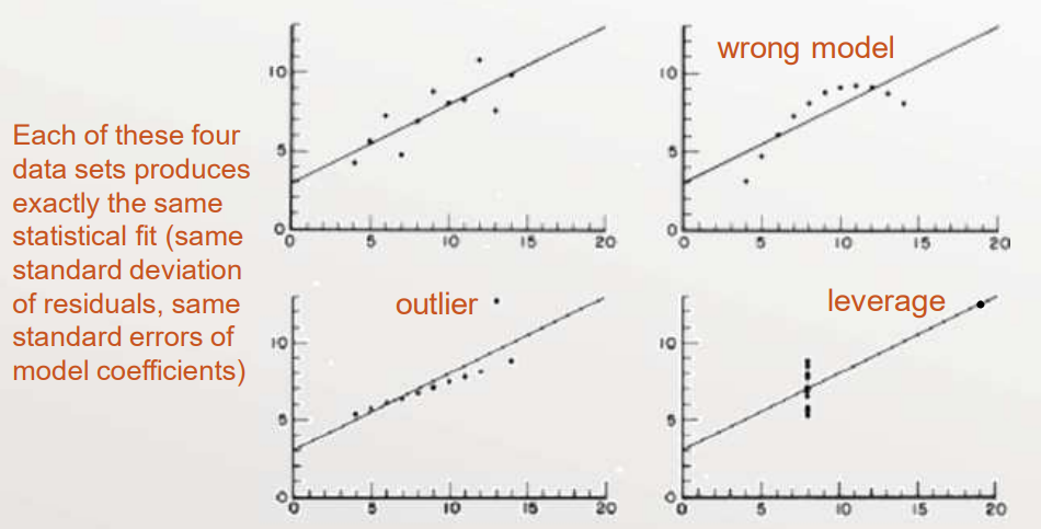
Failed Assumptions – the Anscombe Problems

F. J. Anscombe, “Graphs in Statistical Analysis”, The American Statistician, Vol. 27, No. 1
(Feb., 1973) pp. 17 – 21.

What Happens When OLS Assumptions are Violated?

At best, the regression becomes inefficient
— Do the assumptions in OLS regression holdThe uncertainty around the estimates is larger than you think: $\operatorname{var}[\hat{\theta}]$ for some parameter $\theta$
At worst, the regression becomes biased
— The results may be misleading: bias $[\hat{\theta}]$
We want small mean square error (MSE)$$\operatorname{MSE}(\hat{\theta})=\operatorname{var}[\hat{\theta}]+(\operatorname{bias}[\hat{\theta}])^{2}$$

Checking Our Assumptions

Regression Diagnostics: checking for violations in any of the OLS assumptions
Topics we'll address:
- Normality of residuals
- Outliers (identically distributed)
- Leverage and influence
- Heteroscedasticity (variation in variance)
- Error in predictor variables
- The wrong model
- Correlated residuals

Fixing Problems

Regression Remediation: changing our regression to address diagnostic problems
Topics we'll address:
- Outlier removal or adjustment
- Data transformation
- Weighted regression
- Total regression
- Model building
- Autocorrelation analysis

Response surface methodology

链接

Data and Measurement

Data Example

Process Modeling

Regression Review

Response surface methodology

You Might Also Like

半导体物理-柴常春

光通信

Multisim

Leave a Reply Cancel reply