Optimization Toolbox
不要修改本文字体
非线性拟合lsqcurvefit、nlinfit-CSDN
非线性拟合方法的MATLAB实现-科学网
Set Optimization Options
Create or modify optimization options structure.
Options Table如下
TolFun(fminsearch): The termination tolerance for the function value. The default value is 1.e-4.
TolX(fminbnd, fminsearch, fzero, lsqnonneg): is a lower bound on the size of a step(步长大小的下界).The default value is 1.e-4, except for fzero, which has a default value of eps (= 2.2204e-16), and lsqnonneg, which has a default value of 10*eps*norm(c,1)*length(c).
PlotFcns(fminbnd, fminsearch, fzero): Plot information on the iterations of the solver. The default is [] (none).选择有三种
@optimplotxplots the current point@optimplotfvalplots the function value@optimplotfunccountplots the function count (not available for fzero)
MaxIter(fminbnd, fminsearch): The maximum number of iterations allowed. The default value is 500 for fminbnd and 200*length(x0) for fminsearch.
MaxFunEvals(fminbnd, fminsearch): The maximum number of function evaluations allowed. The default value is 500 for fminbnd and 200*length(x0) for fminsearch.
OutputFcn(fminbnd, fminsearch, fzero): Display information on the iterations of the solver. The default is [] (none).?
Display(fminbnd, fminsearch, fzero, lsqnonneg): A flag indicating whether intermediate steps appear on the screen.
(a)'notify' (default) displays output only if the function does not converge.
(b)'iter' displays intermediate steps (not available with lsqnonneg).
(c)'off' or 'none' displays no intermediate steps. 'final' displays just the final output.
FunValCheck(fminbnd, fminsearch, fzero): Check whether objective function values are valid.
(a)'on' displays an error when the objective function or constraints return a value that is complex or NaN.
(b)'off' (default) displays no error.
(1) 在进行优化的时候,用户可以指定目标函数和/或约束函数。每当这些函数被调用一次,就算一个function evaluation。在一次iteration过程中,往往会有若干中间步骤,所以一次迭代会有多次function evaluation。所以这个参数不等同于迭代次数,而往往大于迭代次数。最大迭代次数的参数是MaxIter。
(2) Unlike other solvers, fminsearch stops when it satisfies both TolFun and TolX.
(3) eps是Matlab浮点数的相对精度,对于数值X,如果2^E <= abs(X) < 2^(E+1), 对于double型数值X,eps(X) = 2^(E-52) 对于single型数值X,eps(X) = 2^(E-23)。
(4) 注意x=(-3:0.1:3)+eps;y=sin(x)./x; plot(x,y)中eps的用处。
(5) Generally, set the TolFun and TolX tolerances to well above eps, and usually above 1e-14. Setting small tolerances does not guarantee accurate results. Instead, a solver can fail to recognize when it has converged, and can continue futile iterations. A tolerance value smaller than eps effectively disables that stopping condition. This tip does not apply to fzero, which uses a default value of eps for TolX.
常用例子:
x = fminsearch(fun,x0,options)
options = optimset('Display','iter');
%display output from the algorithm at each iteration, set the Display option to 'iter':
Output Structure
The output structure includes the number of function evaluations, the number of iterations, and the algorithm. The structure appears when you provide fminbnd, fminsearch, or fzero with a fourth output argument, as in
[x,fval,exitflag,output] = fminbnd(@humps,0.3,1);
optimset
Create or modify optimization options structure
(a) Create Nondefault Options
Set options for fminsearch to use a plot function and a stricter stopping condition than the default.
options = optimset('PlotFcns','optimplotfval','TolX',1e-7);
fun = @(x)100*((x(2) - x(1)^2)^2) + (1 - x(1))^2; % Rosenbrock's function
x0 = [-1,2];
[x,fval] = fminsearch(fun,x0,options)
(b) Create Default Options for Solver
options = optimset('fzero'); %Create a structure containing the default options for the fzero solver.
tol = options.TolX % View the default value of the TolX option for fzero.
(c) Modify Options
oldopts = optimset('TolFun',1e-6); % Set options to use a function tolerance of 1e-6.
options = optimset(oldopts,'PlotFcns','optimplotfval','TolX',1e-6); % Modify options in oldopts to use the 'optimplotfval' plot function and a TolX value of 1e-6.
disp(options.TolFun); % View the three options that you set.
disp(options.PlotFcns);
disp(options.TolX);
(d) Modify 算法
比如在fmincon函数中opts = optimset('algorithm','sqp')
一元函数最小值fminbnd
实例
(1) sin函数在区间0-2pi的最小值;
(2) 二次函数x^2-2x-2的最小值,并作图;
fminbnd的关键词是:一元/有约束(边界条件)/连续(算法依赖求导或微分)/局部最优解。
算法:黄金分割法/抛物插值法
opts = optimset('display','iter');
%opts.TolX = 1e-2; %change this paramter
fminbnd(@sin,0,2*pi,opts)

%%
%  Func-count     x          f(x)         Procedure
%     1        2.39996      0.67549        initial
%     2        3.88322     -0.67549        golden
%     3        4.79993    -0.996171        golden
%     4        5.08984    -0.929607        parabolic
%     5        4.70582    -0.999978        parabolic
%     6         4.7118           -1        parabolic
%     7        4.71239           -1        parabolic
%     8        4.71236           -1        parabolic
%     9        4.71242           -1        parabolic
%
% Optimization terminated:
% the current x satisfies the termination criteria using OPTIONS.TolX of 1.000000e-04
% ans =
%
%     4.7124

 %%
 f = @(x)x.^2-2*x-2;
 fplot(f),grid on
 fminbnd(f,-1000,1000)
 %fminbnd(f,-1000,0)
 [x,fval,ex,msg]= fminbnd(f,-1000,1000)  % ex =1 menas conervge
 hold on
 plot(x,fval,'ro')
多元函数最小值fminsearch函数
Find minimum of unconstrained multivariable function using derivative-free method. It is a nonlinear programming solver. Searches for the minimum of a problem specified by \(\min _{x} f(x)\). f(x) is a function that returns a scalar, and x is a vector or a matrix. 基于Nelder–Mead Simplex method算法。
关键词:多元/无约束/直接寻优法(非导数法)
f = @(x)x.^4 -100*x.^2-10*x+1
ezplot(f, [0, 10])
fminsearch
例子1:求解(x-1)^2+1的最小值
f = @(x)(x-1).^2+3;
fminsearch(f,0) % 0作为初始值,去寻找最小f,输出最小的f时对应的x的值
[x, fval]= fminsearch(f,0) % 0作为初始值,去寻找最小f,输出最小的f时对应的x的值以及f
例子2:求解(x-1)^2+y^2+5的最小值
f = @(x,y)(x-1).^2+y.^2+5; % 由自变量x和y定义的匿名函数交给句柄f
objfun = @(x)f(x(1),x(2)); % 用向量x(包含元素x(1)和x(2))去替换之前的自变量x和y
x0 = [10, 10]; % 定义向量的初始值
fminsearch(objfun,x0) % 调用目标函数,以及初始值,输出一个向量
例子3:稍微修改例子2中的代码
f = @(x)(x(1)-1).^2+x(2).^2+5; % 直接用向量x作为函数的自变量
x0 = [10, 10]; % 给定向量x的初始值
[x,fval,exitflag,output] = fminsearch(f,x0)
结果为:
x =1.0000 -0.0000 %目标函数最小值时对应的向量x
fval =5.0000 % 目标函数的最小值
exitflag =1 % 是否满足收敛要求,为1就满足
output = % 结构体,输出和迭代过程有关的信息
struct with fields:
iterations: 46 %迭代次数
funcCount: 90 %函数计算
algorithm: 'Nelder-Mead simplex direct search'
message: 'Optimization terminated:↵ the current x satisfies the termination criteria using OPTIONS.TolX of 1.000000e-04 ↵ and F(X) satisfies the convergence criteria using OPTIONS.TolFun of 1.000000e-04 ↵'
例子4:
fun2 = @(x,y,z)exp((x+y).^2)+(x-1).^2+2*sin(z);
objfun2 = @(x)fun2(x(1),x(2),x(3));
x0 = [1 1 1];
[x,fval,ex,msg ]=fminsearch(objfun2,x0)
注:任何优化函数最后的参数都是选项,例子4中的可以设置opts =[]然后最后一句变为[x,fval,ex,msg ]=fminsearch(objfun2,x0, opts)不改变最后的结果。
带约束多元函数最小值fmincon
关键词:多元/非线性/有约束
算法:
‘interior-point’(default)
'trust-region-reflective'
'sqp'
'sqp-legacy(optimoptions only)'
'active-set'
$$\left\{\begin{array}{l} \mathrm{A}^{*} \mathrm{x} \leqslant \mathrm{b} \\ \mathrm{Aeq}^{*} \mathrm{x}=\mathrm{beq} \\ \mathrm{lb} \leqslant \mathrm{x} \leqslant \mathrm{ub} \\ \mathrm{c}(\mathrm{x}) \leqslant 0 \\ \operatorname{ceq}(\mathrm{x})=0 \end{array}\right.$$
例子(1)
函数exp((x+y)^2)+(x-1)^2的最小值
约束条件:x+y≥1 线性不等式约束,x+2y =1.5 线性等式约束,x≥0.6边界条件
fun = @(x,y)exp((x+y).^2)+(x-1).^2;
objfun = @(x)fun(x(1),x(2));
x0 = [0, 0];
[x,fval] = fminsearch(objfun,x0)  % 没有约束条件

A =[-1 -1]; % -x smaller or equal to -1
b = -1;
Aeq = [1 2];
beq = 1.5;
lb =[0.6 -inf];
ub =[]; % or ub =[inf inf];
[x, fval] = fmincon(objfun,x0,A,b,Aeq,beq,lb,ub) % 注意输入值的顺序
例子(2)
函数exp((x+y)^2)+(x-1)^2的最小值
约束条件:x^2+y^2≥1 非线性的不等式约束,x^2+2y^2=1.5非线性等式约束
fun = @(x,y)exp((x+y).^2)+(x-1).^2;
objfun = @(x)fun(x(1),x(2));
x0 = [0, 0];


A =[];
b = [];
Aeq = [];
beq = [];
lb =[];
ub =[];
% opts = optimset('algorithm','sqp') %修改算法
% opts = optimoptions('fmincon','algorithm','sqp') %效果和上一行一样
[x, fval] = fmincon(objfun,x0,A,b,Aeq,beq,lb,ub,@confun,opts)


function [c,ceq] = confun(x)
c = -x(1).^2-x(2).^2+1;
ceq=x(1).^2+2*x(2).^2-1.5;
end
无约束多元函数最小值fminunc
实例
(1)函数(x-1)²+y²+5 最小值;
(2)函数 exp((x+y)²)+(x-1)²+2*sin(z)最小值;
关键词:无约束/非线性/多元函数
算法:quasi-newton Algorithm和trust-region Algorithm
f = @(x,y)(x-1).^2+y.^2+5;
objfun = @(x)f(x(1),x(2));
x0 = [10, 10];
[x, fval] = fminsearch(objfun,x0) %loca min
[x, fval] = fminunc(objfun,x0)


%%
fun2 = @(x,y,z)exp((x+y).^2)+(x-1).^2+2*sin(z);
objfun2 = @(x)fun2(x(1),x(2),x(3));
x0 = [1 1 1];
opts =[];
[x,fval,ex,msg]=fminsearch(objfun2,x0,opts)
[x,fval,ex,msg]=fminunc(objfun2,x0,opts)  %函数运算次数更少
如何进一步减少函数运算次数?(同样求解问题2)
x0 = [1 1 1];
opts = optimoptions('fmincon','specifyobjectivegradient','true')
[x,fval,ex,msg]=fminunc(@objfun3,x0,opts)

function [fun,gfun]=objfun3(x)  %计算梯度的时候直接使用我们添加的公式计算,减少了函数计算的次数
fun = exp((x(1)+x(2)).^2)+(x(1)-1).^2+2*sin(x(3));
g1=  % 对x(1)求偏导数
g2=  % 对x(2)求偏导数
g3=  % 对x(3)求偏导数
gfun=[g1,g2,g3]
半无限约束多元函数最小值fseminf(待补充)
1.实例
(1)min f(x)=x²
st. x+2-exp(t-2)≤0,其中 0≤t≤1
(2)min f(x,y)=x²+y²
st. x+2-exp(t - 2)≤0,y+2-sin(t)≤0,其中 0≤t≤1
问题定义:半无限约束多元非线性函数优化问题(带额外参数的约束条件)$$\begin{aligned} &\min \mathrm{f}(\mathrm{x})\\ &\text { st. }\\ &\left\{\begin{array}{l} \mathrm{A}^{*} \mathrm{x} \leqslant \mathrm{b} \\ \mathrm{Aeq}^{*} \mathrm{x}=\mathrm{beq} \\ \mathrm{lb} \leqslant \mathrm{x} \leqslant \mathrm{ub} \\ \mathrm{c}(\mathrm{x}) \leqslant 0 \\ \operatorname{ceq}(\mathrm{x})=0 \\ \mathrm{~K}(\mathrm{x}, \mathrm{t}) \leqslant 0 \end{array}\right. \end{aligned}$$
关键词:半无限约束/带额外参数的约束条件
多目标函数最优点达到问题fgoalattain
实例
(1)函数[sin((3π/2)x),x²+1],目标[0,1.5],权重[1,1](同等重要),求 x;
(2)函数[sin((3π/2)x),(x+y)²+cos(yπ)] ,目标[0,1.5],权重[1,1],st. x+y≤1,求 x,y;
问题定义
多目标函数最优点达到问题$$\begin{aligned} &\min \beta\\ &\text { st. }\\ &\mathrm{F}(\mathrm{x}) \text { -weight }^{*} \beta \leqslant \text { goal }\\ &\left\{\begin{array}{l} \mathrm{A}^{*} \mathrm{x} \leqslant \mathrm{b} \\ \mathrm{Aeq}^{*} \mathrm{x}=\mathrm{beq} \\ \mathrm{lb} \leqslant \mathrm{x} \leqslant \mathrm{ub} \\ \mathrm{c}(\mathrm{x}) \leqslant 0 \\ \operatorname{ceq}(\mathrm{x})=0 \end{array}\right. \end{aligned}$$
关键词:多值函数/给出目标值和权重
算法: 'active-set'
多目标函数最大值最小值问题fminimax
实例
min max(F(x)),F(x)=[sin(x)+cos(x),sin(x)-cos(x)]
问题定义
多目标函数最大值的最小值问题$$\begin{aligned} &\min \max \mathrm{F}(\mathrm{x})\\ &\text { st. }\\ &\left\{\begin{array}{l} \mathrm{A}^{*} \mathrm{x} \leqslant \mathrm{b} \\ \mathrm{Aeq}^{*} \mathrm{x}=\mathrm{beq} \\ \mathrm{lb} \leqslant \mathrm{x} \leqslant \mathrm{ub} \\ \mathrm{c}(\mathrm{x}) \leqslant 0 \\ \operatorname{ceq}(\mathrm{x})=0 \end{array}\right. \end{aligned}$$
关键词:多值函数
线性规划linprog
实例,已知$$\left\{\begin{array}{l}
2 x-y \leqslant 2 \\
x-y \geqslant-1 \\
x+y \geqslant 1
\end{array}\right.$$求 z=2x+3y的最大值
问题定义:线性规划 (LP,linear programming)$$\begin{aligned} &\min \mathrm{f}^{\mathrm{T}} \mathrm{X}\\ &\text { st. }\\ &\left\{\begin{array}{l} \mathrm{A}^{*} \mathrm{x} \leqslant \mathrm{b} \\ \mathrm{Aeq}^{*} \mathrm{x}=\mathrm{beq} \\ \mathrm{lb} \leqslant \mathrm{x} \leqslant \mathrm{ub} \end{array}\right. \end{aligned}$$
关键词:目标函数和约束都是线性的
算法:'dual-simplex' (default)
'interior-point-legacy'
'interior-point'
混合整数线性划 规划 intlinprog
例子
已知\(\left\{\begin{array}{l} x \geqslant 1 \\ x-y+1 \leqslant 0 \\ 2 x-y-2 \leqslant 0 \end{array}\right.\),则\(x^{2}+y^{2}\),则\(x^{2}+y^{2}\)的最小值是?
问题定义
二次规划问题(QP,quadratic programming)$$\begin{aligned} &\min (1 / 2) \mathrm{x}^{\mathrm{T}} \mathrm{Hx}+\mathrm{f}^{\mathrm{T}} \mathrm{x}\\ &\text { st. }\\ &\left\{\begin{array}{l} \mathrm{A}^{*} \mathrm{x} \leqslant \mathrm{b} \\ \mathrm{Aeq}^{*} \mathrm{x}=\mathrm{beq} \\ \mathrm{lb} \leqslant \mathrm{x} \leqslant \mathrm{ub} \end{array}\right. \end{aligned}$$
关键词:二次目标函数/线性约束H 必须正定
算法: interior-point-convex
trust-region-reflective
线性最小二乘问题 lsqlin
实例
(1) 已知\(\left\{\begin{array}{l} \mathrm{x} \geqslant 1 \\ \mathrm{x}-\mathrm{y}+1 \leqslant 0 \\ 2 \mathrm{x}-\mathrm{y}-2 \leqslant 0 \end{array}\right.\),则\( x^{2}+y^{2}\)的最小值是
可以这样思考 C=[1 0
0 1]
d=[0 0]
||Cx-d|| ^2 =x^2+y^2
(2) 数据拟合(将数据拟合问题转化为优化问题)$$\begin{array}{lcccc} \hline & \mathrm{X} 1 & \mathrm{X} 2 & \mathrm{X} 3 & \mathrm{Y} \\ \hline 1 & 1 & 2 & 3 & 3 \\ 2 & -1 & 1 & 5 & 2 \\ 3 & 2 & 0 & 4 & 8 \\ \hline \end{array}$$
问题定义:线性最小二乘问题 $$$\min (1 / 2)\|\mathrm{Cx}-\mathrm{d}\|^{2}$ st. $\left\{\begin{array}{l}\mathrm{A}^{*} \mathrm{x} \leqslant \mathrm{b} \\ \mathrm{Aeq}^{*} \mathrm{x}=\mathrm{beq} \\ \mathrm{lb} \leqslant \mathrm{x} \leqslant \mathrm{ub}\end{array}\right.$$$
关键词:2-范数/线性约束
算法:Trust-Region-Reflective Algorithm
Interior-Point Algorithm
非负线性最小二乘问题lsqnonneg
实例
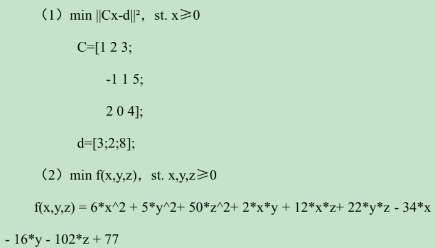 问题定义,非负线性最小二乘问题 $$\begin{aligned} &\min \|\mathrm{C} \mathrm{x}-\mathrm{d}\|^{2}\\ &\text { st. } \mathrm{x} \geqslant 0 \end{aligned}$$
关键词:非负/无约束
非线性函数拟合题 问题 lsqcurvefit
实例1
使用随机数据,拟合函数:$$\mathrm{f}(\mathrm{x})=\mathrm{a}_{1} \mathrm{x}^{2}+\mathrm{a}_{2} \mathrm{x}+\mathrm{a}_{3}+\mathrm{a}_{4} \exp \left(\mathrm{a}_{5} \mathrm{x}\right)$$
xdata=randi(20,1,10);
ydata=xdata.^2+2*xdata+20+0.5*exp(0.1*xdata)+rand;

fun =@(a,xdata)a(1)*xdata.^2+a(2)*xdata+a(3)+a(4)*exp(a(5)*xdata)
a0 =[0 0 0 0 0]
lb=[];
ub =[];
opts=[];
lsqcurvefit(fun,a0,xdata,ydata,lb,ub,opts)
例子中的点比较少,所以也可能出现拟合出的结果与事先设定的值偏差较大的情况。
实例2:对于函数y=a*sin(x)*exp(x)-b/log(x)我们现在已经有多组(x,y)的数据,我们要求最佳的a,b值
%针对上面的问题,我们可以来演示下如何使用这个函数以及看下其效果
x=2:10;
y=8*sin(x).*exp(x)-12./log(x);
%上面假如是我们事先获得的值
a=[1 2];
f=@(a,x)a(1)*sin(x).*exp(x)-a(2)./log(x);
%使用lsqcurvefit
[A,resnorm]=lsqcurvefit(f,a,x,y) %resnorm残差平方和  A是参数
实例3:多自变量+多参数
问题定义:使用最小二乘法求解非线性函数拟合问题\(\min \|\mathrm{F}(\mathrm{a}, \mathrm{xdata})-\mathrm{ydata}\|^{2}\),其中a是未知的系数矩阵(向量),而xdata和ydata是已知的样本数据。
实例4:我自己的例子
x = [t ;T];

fun= @(a,x)a(3)*0.01*exp(-a(5)*0.1*10^12*a(2)*exp(-a(1)*1000./x(2,:)).*x(1,:)./(a(6)*10^14+a(5)*0.1+a(2)*10^12*exp(-10^3*a(1)./x(2,:))))+a(4)*0.1;
a0 =[1.478     1         2.32       2.072        4.989        1.0];
lb = [0.116   1.0   0.1   1.0   0.01   10^(-4)];
ub = [5820   100   50   2.3   10^3   10];

[A,resnorm] = lsqcurvefit(fun,a0,x,F,lb,ub)
关键词:曲线拟合/数据拟合/任意形式函数的拟合
算法:Levenberg-Marquardt 或者 trust-region-reflective
nlinmultifit—同时拟合多组数据
Multiple curve fitting with common parameters using NLINFIT
非线性最小二乘问题lsqnonlin
实例:计算最小值\( \sum_{k=1}^{5}\left(1+\sin (k x)-e^{k y}\right)^{2} \)
问题定义
非线性最小二乘问题(非线性数据拟合)\(\min \|\mathrm{f}(\mathrm{x})\|^{2}\)
关键词:目标函数输入形式/无约束
算法
Levenberg-Marquardt
trust-region-reflective
lsqnonlin
实例
t =[0,120,240,360,480,600,720,840,960,1080,1200,1320,1440,1560,0,120,240,360,480,600,720,840,960,1080,1200,1320,1440,1560,0,120,240,360,480,600,720,840,960,1080,1200,1320,1440,1560,0,120,240,360,480,600,720,840,960,1080,1200,1320,1440,1560,0,120,240,360,480,600,720,840,960,1080,1200,1320,1440,1560,0,120,240,360,480,600,720,840,960,1080,1200,1320,1440,1560,0,120,240,360,480,600,720,840,960,1080,1200,1320,1440,1560];
T =[453.150000000000,453.150000000000,453.150000000000,453.150000000000,453.150000000000,453.150000000000,453.150000000000,453.150000000000,453.150000000000,453.150000000000,453.150000000000,453.150000000000,453.150000000000,453.150000000000,393.150000000000,393.150000000000,393.150000000000,393.150000000000,393.150000000000,393.150000000000,393.150000000000,393.150000000000,393.150000000000,393.150000000000,393.150000000000,393.150000000000,393.150000000000,393.150000000000,363.150000000000,363.150000000000,363.150000000000,363.150000000000,363.150000000000,363.150000000000,363.150000000000,363.150000000000,363.150000000000,363.150000000000,363.150000000000,363.150000000000,363.150000000000,363.150000000000,333.150000000000,333.150000000000,333.150000000000,333.150000000000,333.150000000000,333.150000000000,333.150000000000,333.150000000000,333.150000000000,333.150000000000,333.150000000000,333.150000000000,333.150000000000,333.150000000000,273.150000000000,273.150000000000,273.150000000000,273.150000000000,273.150000000000,273.150000000000,273.150000000000,273.150000000000,273.150000000000,273.150000000000,273.150000000000,273.150000000000,273.150000000000,273.150000000000,253.150000000000,253.150000000000,253.150000000000,253.150000000000,253.150000000000,253.150000000000,253.150000000000,253.150000000000,253.150000000000,253.150000000000,253.150000000000,253.150000000000,253.150000000000,253.150000000000,233.150000000000,233.150000000000,233.150000000000,233.150000000000,233.150000000000,233.150000000000,233.150000000000,233.150000000000,233.150000000000,233.150000000000,233.150000000000,233.150000000000,233.150000000000,233.150000000000];
ydata =[0.229762645914397,0.222313710902021,0.214288496211636,0.208193624335552,0.203204695979430,0.198821613215673,0.195229360710123,0.192307563030905,0.189763818018160,0.187051746446297,0.185111497449830,0.183086460937727,0.181349668866581,0.179468533707833,0.229762645914397,0.221960578175988,0.214599892748681,0.208574024130363,0.203633417152188,0.199398830916528,0.195670356621565,0.192396236227707,0.189655448317237,0.186847148351944,0.184720384114189,0.182574996381243,0.180607095250557,0.178630092316273,0.229762645914397,0.222654941496702,0.215488195946841,0.209528376097749,0.204735759433500,0.200369765466016,0.196800077581859,0.193552441849634,0.190508302858360,0.188118744880483,0.185799500414241,0.183464848259145,0.181617020998089,0.179645583045470,0.229762645914397,0.224412775668780,0.218480695065428,0.213587881588155,0.209135191340965,0.205509603771606,0.202075603485780,0.199291650751184,0.196404040594266,0.194125742062212,0.192140957721524,0.189960347271881,0.188215669939335,0.186822583493463,0.229762645914397,0.225331242144553,0.220307504816169,0.216359163162286,0.213014798083167,0.210075200996487,0.206622040660046,0.204058322074751,0.201940220694598,0.199549439056935,0.197509416379188,0.195538692631521,0.193514996078180,0.191914617823535,0.229762645914397,0.225654406107011,0.221160218794630,0.216888640999863,0.213947601138061,0.210926525140879,0.207828786876165,0.205187992448073,0.203166621076933,0.201529725448822,0.199946533860066,0.197900294885601,0.196286363799515,0.194895980958621,0.229762645914397,0.224840223240085,0.220410622544208,0.216905007679472,0.213668095860012,0.210694389067032,0.208222607340045,0.206336807798863,0.204120770324228,0.201950570885790,0.200427299387014,0.198244470058252,0.196877246813517,0.195605982187081];

x = [t;T];

fun= @(a)a(3)*exp(-a(5)*(10^14*exp(-a(1)./x(2,:))+a(2)).*x(1,:)./(a(2)+a(6)+a(5)+10^14*exp(-a(1)./x(2,:))))+a(4)-ydata;
aGuess = [100  10^12    0.06  0.170   0.002   2.584*10^13];
aFit = lsqnonlin(fun,aGuess);