Integral transform

【积分变换】(integral transform) maps a function from its original function space into another function space via integration, where some of the properties of the original function might be more easily characterized and manipulated than in the original function space. The transformed function can generally be mapped back to the original function space using the inverse transform.

傅立叶级数和表示论有什么关系？

 

群表示论是物理系学生能接触到的数学里最美的分支之一。读研时一个晚上突然发现物理学里那些常用的正交函数族、Fourier变换与群表示论间有非常漂亮的联系。

尽管积分变换的性质千差万别，但是它们都是线性算子。

任意积分变换都具有如下的形式：$$ (T f)(u)=\int_{t_{1}}^{t_{2}} f(t) K(t, u) d t $$输入函数为\( f(t)\)，输出函数为\(Tf(u)\)，自变量也从\(  t\)变为\(u\)。\(T\)为积分变换算子，同时也是线性算子。在矩阵形式的线性代数，最常见的形式是将一个矩阵(线性算子)作用在一个列向量上，那么得到的仍旧是

深入理解傅里叶变换

参考资料：
(1) 傅里叶变换、拉普拉斯变换、Z 变换的联系是什么？为什么要进行这些变换—知乎  微信公众号

拉普拉斯变换

见微分方程笔记，同时阅读下面的连接：1    2

 

 

小波变换

Overview: Why wavelet Transform?

FT的局限性

小波理论的研究主要是从上世纪七十年代开始的。

For FT, no frequency information is available in the time-domain signal, and no time information is available in the Fourier transformed signal. The natural question that comes to mind is that is it necessary to have both the time and the frequency information at the same time? The FT gives the frequency information of the signal, which means that it tells us how much of each frequency exists in the signal, but it does not tell us when in time these frequency components exist. This information is not required when the signal is so-called stationary.

对于\( x(t) = \cos(2 \pi \cdot 10 t) + \cos(2 \pi \cdot 25 t) + \cos(2 \pi \cdot 50 t) + \cos(2 \pi \cdot 100 t) \)这样一个stationary信号做FFT可以得到最左侧的图，四个峰分别对应10、25、50和100 Hz。靠右侧的两个图，是non-stationary signal，不同频率的信号在不同的区间依次独立出现，但是其FFT结果和最左侧的几乎一样。稍微有点区别的地方是出现了一些ripples(涟漪)，they are due to sudden changes from one frequency component to another, which have no significance in this text. 另外就是这四个spikes频率的幅值和和左图的也不一样 (which can always be normalized)，这是因为不同频率的持续时间不一样。总之，下面的图表面时域相差很大的两个信号，可能频谱图一样，要准确描述这种non-stationary signal，FT是不够用的。

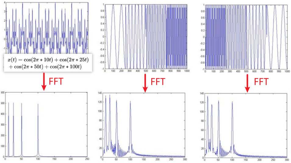
对于stationary信号，每个确定的频率分量，其在任意时刻的贡献都是相同的，但是上面的non-stationary信号，不同时刻(或者说时间区间)，有时某个频率分量有贡献，有的时候可能没贡献。

The FT gives the spectral content of the signal, but it gives no information regarding where in time those spectral components appear. Therefore, FT is not a suitable technique for non-stationary signal, 除非我们不关心non-stationary信号不同频率分量是什么时候出现的。

现实中，有的信号是stationary，有的是non-stationary。前者多为人造出来的；几乎所有的生物信号都属于后者，比如心电图、脑电图、肌电图，多普勒效应导致的不同时刻的频率变化的信号，也属于后者。

When the time localization of the spectral components (frequency components) are needed, a transform giving the TIME-FREQUENCY REPRESENTATION of the signal is needed.

终极方案——The Wavelet Transform

小波变换提供了原始信号的【时频表示】(time-frequency representation, TFR)，即同时提供时间和频率的信息。当然了，其他的一些变换，比如【短时傅里叶变换】(Short-time Fourier Transform, STFT)、【维格纳分布】(Wigner Distribution Function)。

Often times a particular spectral component occurring at any instant can be of particular interest. In these cases it may be very beneficial to know the time intervals these particular spectral components occur. 小波变换 is capable of providing the time and frequency information simultaneously, hence giving a time-frequency representation of the signal. 波变换是作为STFT的替代品而开发的，或者说是为了克服STFT的一些与分辨率相关的问题。

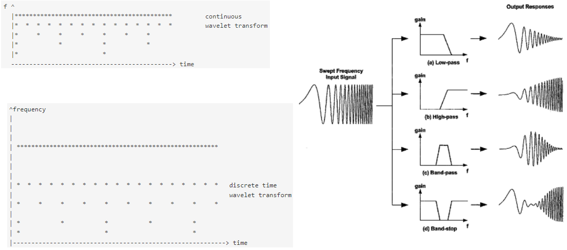
实例：Se pass the time-domain signal from various high pass and low pass filters, which filters out either high frequency or low frequency portions of the signal. This procedure is repeated, every time some portion of the signal corresponding to some frequencies being removed from the signal. 假设我们有一个原始信号，其最高频率为1000 Hz，我们不断对低频部分采用二分法。即第一步将原信号分为0~500 Hz和500~1000Hz两部分；第二步将第一步得到的低频部分分为0~250 Hz和250~500Hz两部分；第三步将第二步得到的低频部分分为0~125 Hz和125~250Hz两部分；不断重复此【decomposition】过程，直到达到a pre-defined certain level。Then we have a bunch of signals, which actually represent the same signal, but all corresponding to different frequency bands. 将滤波得到的各种信号曲线放在同一张图中，即可得到3-D graph，三个轴分别代表时间、频率和幅值。于是我们可以知道什么频率的信号，在什么时候的幅值最大。

注意事项：

• 在分频的过程就是让time-domain signal通过various highpass and low pass filters，filters should satisfy some certain conditions, so-called 【admissibility condition】。
• 【uncertainty principle】: 频率和时间之间的不确定关系\( \Delta t \Delta f \geq \displaystyle\frac{1}{4 \pi}\)
  we cannot exactly know what frequency exists at what time instance, but we can only know what frequency bands exist at what time intervals. 我们能做的最好的就是研究what spectral components exist at any given interval of time. This is a problem of resolution, and it is the main reason why researchers have switched to WT from STFT. STFT gives a fixed resolution at all times, whereas WT gives a variable resolution as follows:

• higher frequencies are better resolved in time，但是在frequency domain的分辨率不好;
• lower frequencies are better resolved in frequency，但是在time domain的分辨率不好.

 

Fundamentals: The Fourier transform and the short term Fourier transform, resolution problems

先回顾一下FT及其逆变换$$ \begin{aligned} &X(f)=\int_{-\infty}^{\infty} x(t) \cdot e^{-2 j \pi f t} d t \\ &x(t)=\int_{-\infty}^{\infty} X(f) \cdot e^{2 j \pi f t} d f \end{aligned} $$对于FT，原始信号\(x(t)\)和一个指数项相乘，at some certain frequency \(f\), and then integrated over ALL TIMES !!! 因此FT得到的频域信号\(X(f)\) is calculated for every value of \(f\).

注意：

• FT频谱计算的积分区间是从负无穷到正无穷，覆盖整个信号区间，即对所有任意时刻的频率分布做了累加处理，所以只会告诉你每个频率分量的贡献是多少，但是不会告诉你任意频率分量出现的位置。某个频率分量出现在\(t_1\)或者\(  t_2\)，堆FT频谱具有相同的贡献。This is why Fourier transform is not suitable if the signal has time varying frequency, i.e., the signal is non-stationary.
• 在使用FT之前，知道信号是否是stationary很重要。

【STFT】：其实就是通过加窗的方法，把整个时域过程分解成无数个等长的小过程，每个小过程近似平稳，再傅里叶变换，就知道在哪个时间点上出现了什么频率了。对对于上一章节的图中的信号做STFT(更准确地说是STFFT)，就会看到10Hz, 25 Hz, 50 Hz, 100 Hz四个频域成分及其出现的时间。

但是这种处理方法还是存在一个问题，即如何选择窗的大小：对于【窗口函数】\(\omega \)，the width of this window must be equal to the segment of the signal where its stationarity is valid.

假设窗口函数的宽度为\(T\)，那么最开始的时候，窗口函数的中心位置是在\(t=0\)，也就是说只有右侧的部分和信号有重叠，也即原始信号起始的\(T/2\)时间范围内的信号is being chosen, with the appropriate weighting of the window (if the window is a rectangle, with amplitude "1", then the product will be equal to the signal)，信号函数和窗口函数的乘积is assumed to be just another signal, whose FT is to be taken。第二步，就是将窗口函数移动\(t_1\)，乘积再做FT。重复此过程，直到the end of the signal is reached by shifting the window。用公式总结如下：$$STFT_X^{(\omega)}(t',f) = \int_t \left[ x(t) \cdot \omega^*(t - t') \right] \cdot e^{-j 2 \pi f t} dt$$其中\(\omega(t)\)表示窗口函数，\(*\)星号表述复共轭，\(t'\)为【Translation Parameter】，也是time localization。

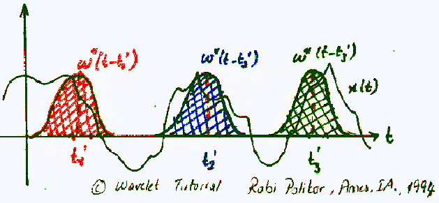
上图中的，红/绿/蓝分别表示窗口函数(高斯峰)分别在\(t_1^\prime\)/\(t_2^\prime\)/\(t_3^\prime\)时刻。窗口函数，扫过整个信号区间，就可以得到时频表示TFR，下面举例说明。

实例：一个non-stationary信号，存在四个250 ms intervals，频率依次为300 Hz，200 Hz，100 Hz，50Hz；下图是其原始信号和STFT后得到的TFR：

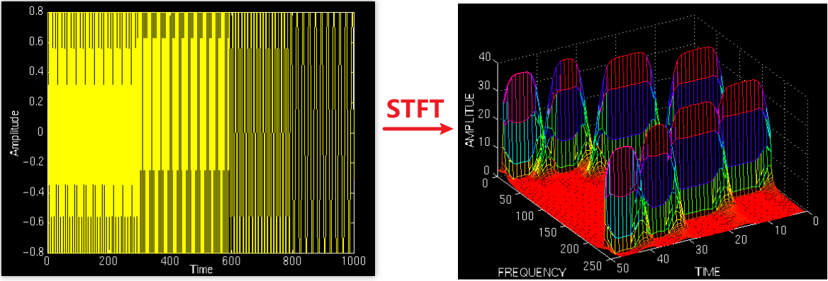
注：Please, ignore the numbers on the axes, since they are normalized in some respect, which is not of any interest to us at this time. Just examine the shape of the time-frequency representation.

分析：

• 由于STFT只是加了窗的FT，而一个实数信号的FT总是对称的，所以TFR从频率轴看是对称的也很正常。非要深究的话，这种对称特性和【负频率】有关，这是一个odd concept which is difficult to comprehend，这个概念在我们这里并不重要。
• 单看一半的图，存在四个peaks，分别对应不同的频率分量，而且它们 are located at different time intervals along the time axis。似乎我们已经得到一个完美的TFR结果？Not really!!!
• 存在的问题：还是测不准原理在捣乱，时间和频率之间的不确定性。one cannot know what spectral components exist at what instances of times. 这个问题和窗口函数的宽度有关。

FT和STFT对比：

• 对于FT，对频域信号，并不存在频率分辨率的问题，因为我们确切地知道存在哪些频率，对于时域信号，也不存在时间分辨率的问题，因为我们确切地知道每个时刻的信号值。但是，频域信号中的时间分辨率、时域信号的频率分辨率都为零；即研究频域信号某一确定频率的时间演化，或者研究某一确定时间的频率演化都是没有任何意义的。FT中的核函数\(e^{-i \omega t}\)让我们获得完美的分辨率，这是因为核本身就是一个无限长的窗口。
• 在STFT中，窗口宽度是有限的，每次只覆盖原始信号的一部分，所以频率分辨率不如FT，或者说分辨率变差，也就是说我们将不再知道某个确定的频率分量， we only know a band of frequencies that exist。
  
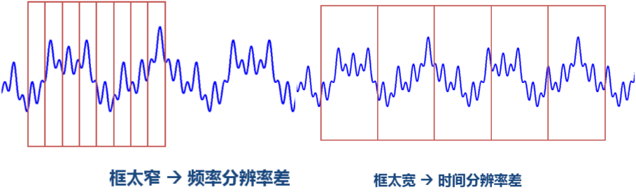
  • 窄窗，时间分辨率高，频率分辨率低；
  • 宽窗，时间分辨率低，频率分辨率高；

实例：下面用四个不同的window作用在相同的信号上，看结果有什么不同。The window function we use here is simply a Gaussian function in the form: \( e^{-a \left( \frac{t^2}{2} \right)}\)，其中的\(a\) determines the length of the window. 下图是不同\(a\)值对应的窗口形状：

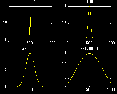
对于第一个很窄串口函数，STFT的时间分辨率很高，但是相对而言频率分辨率就比较差。下图是上面四个窗口函数作用下的STFT结果：

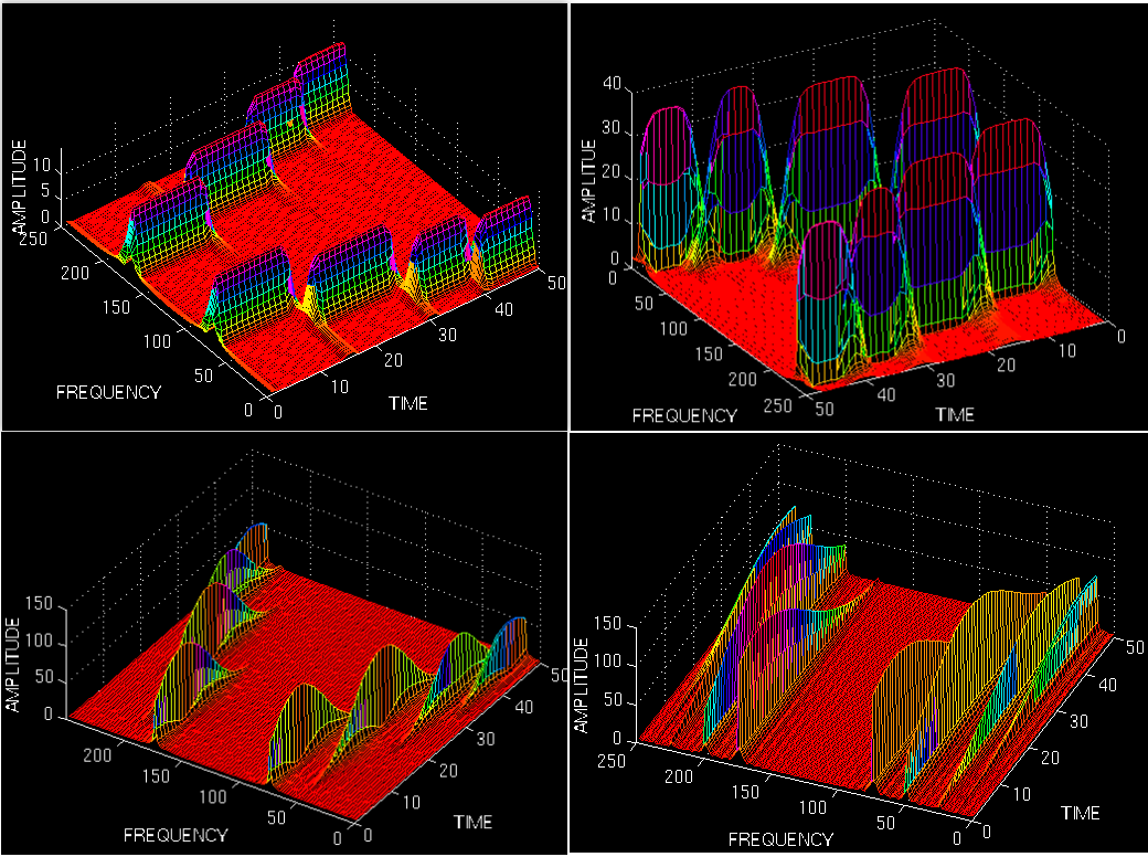
第一张图，时间分辨率很好，但是从左侧看，频率分辨率不太好(呈现展宽)；最后一张图，从左侧的分辨率轴看，展宽很小，表示频率分辨率高，但是从时间轴看，几个频率分量都叠在一起，即时间分辨率很差。

如何选取窗口函数的宽度？
The answer, of course, is application dependent: If the frequency components are well separated from each other in the original signal, than we may sacrifice some frequency resolution and go for good time resolution, since the spectral components are already well separated from each other. However, if this is not the case, then a good window function, could be more difficult than finding a good stock to invest in.

下面将祭出杀器：The Wavelet transform (WT) solves the dilemma of resolution to a certain extent.

 

Multiresolition Analysis: The continuous wavelet transform

Multiresolution Analysis

【Multiresolution Analysis】(MRA): analyzes the signal at different frequencies with different resolutions. 虽然存在时间-频率的不确定性原理，但是我们可以通过MRA这种方法来分析信号。这种方法，every spectral component is not resolved equally as was the case in the STFT。其特点如下：

• give good time resolution and poor frequency resolution at high frequencies;
• give good frequency resolution and poor time resolution at low frequencies.

这种处理方式很合理，特别适用于高频信号-short duration，低频信号-long duration的情况。幸运的是，the signals that are encountered in practical applications are often of this type. 如上图所示，中间一小段表现出高频，而低频信号throughout the entire signal。

 

The Continuous Wavelet Transform

【连续小波变换】(CWT)是作为STFT的替代方案而发展起来的，主要是想解决STFT过程中的分辨率问题。CWT和STFT有点类似，CWT中the signal is multiplied with a function，and the transform is computed separately for different segments of the time-domain signal. CWT和STFT的不同之处在于：

• The Fourier transforms of the windowed signals are not taken, and therefore single peak will be seen corresponding to a sinusoid, i.e., negative frequencies are not computed.
• The width of the window is changed as the transform is computed for every single spectral component, which is probably the most significant characteristic of the wavelet transform.
• CWT得到的结果并没有频率参数，instead, we have 【scale parameter】 which is defined as \(\displaystyle\frac{1}{\text{frequency}}\).

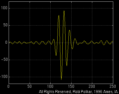
CWT的公式如下：$$CWT_x^\psi(\tau,s) = \Psi_x^\psi(\tau,s) = \frac{1}{\sqrt{|s|}} \int x(t) \psi^* \left( \frac{t - \tau}{s} \right) dt$$其中\(\tau\)和\(s\)分别为translation parameter和scale parameter；\(\psi(t)\)为transforming function，也被称作【mother wavelet】，it gets this name due to two important properties of the wavelet analysis as explained below:

• wavelet的意思是a small wave，这里的"小"指的是窗口函数的有限宽度(【紧支撑】compactly supported)，-let是后缀，比如droplet水滴，booklet小册子，leaflet小树叶；
• 这里的"波"指的是function is oscillatory；
• The term mother implies that the functions with different region of support that are used in the transformation process are derived from one main function, or the mother wavelet. In other words, the mother wavelet is a prototype for generating the other window functions.

用最通俗的话来说，compact support是这样的，对于函数\(f(x)\)，如果自变量\(x\)在\(0\)附近的取值范围内，\(f(x)\)能取到值，而在此之外，\(f(x)\)的取值为\(0\)，那么这个函数\(f(x)\)就是禁支撑函数，而这个\(0\)附近的取值范围就叫作【紧支撑集】，比如在\([-1,1]\)之间的高斯函数。

 

The Scale

这里的scale和地图中用到的比例尺的概念很像。和地图类似，小波变换中大的scale意味着a non-detailed global view (of the signal)，小的比例尺意味着a detailed view。Similarly, in terms of frequency, low frequencies (high scales) correspond to a global information of a signal (that usually spans the entire signal), whereas high frequencies (low scales) correspond to a detailed information of a hidden pattern in the signal (that usually lasts a relatively short time). Cosine signals corresponding to various scales are given as examples in the following figure.

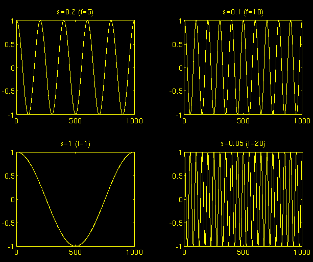
对于现实中绝大多数信号，低频分量往往覆盖整个信号区间，持续时间长，而高频分量表现为short bursts or spikes，持续时间短。从scale的角度看，high scales (low frequencies) usually last for the entire duration of the signal.

Scaling(缩放比例)从数学的角度看，该数值大意味着信号在时间域stretch out，数值小意味着信号compressed。上面的四个函数都是从同一个余弦函数演化而来的，唯一的差异就在与scale的选取。我们知道对于函数\(f(t)\)来说，\(f(st)\)表示corresponds to a contracted (compressed) version of \(f(t)\) if \( s>1\)；但是在CWT中，\(s\)是分母，所以这里正好反过来，即大的\(s>1\)表示信号stretch out。

Computation of the CWT

Multiresolition Analysis: The discrete Wavelet Transform

小波：只在有限时间内有非零值，而在其它所有的时间内都是零。

傅里叶变换是把一个信号通过不同频率的正(余)弦波的线性组合进行表达，这样我们不能找到原始信号中的时域信息。小波变换是把原始信号通过不同时间、不同胖瘦的小波的组合进行表达，这样我们就能知道任意频率组分在不同时刻的的瞬时幅值是多少，能够反映时频特性，即时频分析。

傅里叶变换给出的是：频率-幅值
小波变换给出的是：时间-频率-幅值

参考资料：
(1) The Wavelet Tutorial—The Engineer's Ultimate Guide to Wavelet Analysis
(2) 形象易懂讲解算法I——小波变换—知乎
(3) 小波变换的通俗解释—博客园
(4) 小波变换为什么小—珂学原理