MIT-微分方程-matlab – 历史的进程

欧拉方法ODE1

问：什么是显式解(explicit solution)和隐式解(implicit solution)？
答：可以写成 $y = f (x)$ 的叫作显式解；只能写成 $f (x, y) = C$ 的叫作隐式解，隐式解是方程的形式，但这个方程能确定这个函数。

问：什么是ODE(Ordinary differential equation)和PDE(Partial differential equation)？
答：ODE是常微分方程，PDE是偏微分方程。这里我们将讨论的是ODE常微分方程。

问：什么是函数句柄(function handle)？
答：
(a) 例子
F=@(t,y).06*y-t %这里的.06就是0.06，我们输入t和y值，然后按公式计算
比如F(1,2) 得到的结果为0.06*1-2= -0.8800

(b) 例子(logisctic equation)
a=2;
b=3;
F=@(t, y)a*y-b*y^2

问：什么是欧拉方法ODE1？
答：
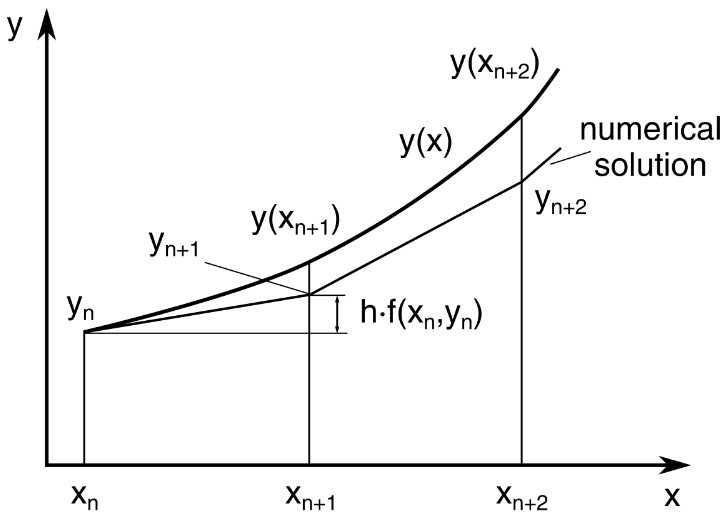欧拉方法 $y^{'} (t) = f (t, y (t)), y (t_{0}) = y_{0}$ 我们知道某一点的导数值和函数值，就可以按照类似泰勒展开形式，只保留一阶导数项。根据 $t_{n + 1} = t_{n} + h$ 有 $y_{n + 1} = y_{n} + h f (t_{n}, y_{n})$

先展示一下ODE1的函数

function yout = ode1(F,t0,h,tfinal,y0)
% ODE1  A simple ODE solver.
%   yout = ODE1(F,t0,h,tfinal,y0) uses Euler's
%   method with fixed step size h on the interval
%      t0 <= t <= tfinal
%   to solve
%      dy/dt = F(t,y)
%   with y(t0) = y0.

%   Copyright 2014 - 2015 The MathWorks, Inc.

   y = y0;
   yout = y;
   for t = t0 : h : tfinal-h
      s = F(t,y);
      y = y + h*s;
      yout = [yout; y];  %每次得到的新的y都放在yout后面拼接起来
   end

例子1 $\begin{aligned} y^{'} = 2 y \\ y (0) = 10 \\ 0 \leq t \leq 3 \end{aligned}$ 求解的代码

F=@(t,y) 2*y;
t0=0;
h=1;
tfinal=3;
y0=10;
ode1(F,t0,h,tfinal,y0)

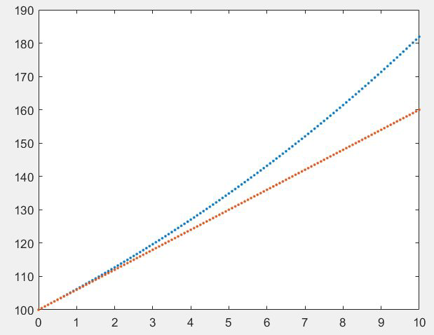
例子2: 用ODE1求复利(compound interest )
假设条件为，初始存入100美元，每年的年利率为6%，每个月底取出所有的本息然后再存进去，如此操作总共12年，求每一个月底的账户金额。

代码如下：

F=@(t,y) .06*y;  %
t0=0;
h=1/12;
tfinal=10;
y0=100;
compound=ode1(F,t0,h,tfinal,y0)
format bank  %取两位小数，分别对应美元和美分
t=(0:h:tfinal)';   %转置一下
simple=y0+100*0.06*t;
plot(t,[compound,simple],'.')  %对比两种存钱方法

中间点法ODE2

问：什么是ODE2方法(midpoint method)？
答：
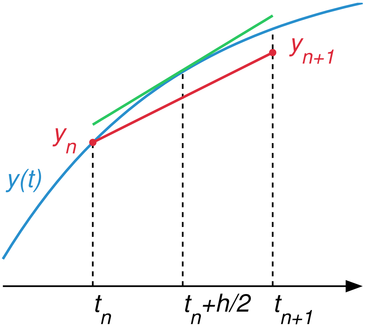ODE1的方法是用个所在点的斜率，推导下一个点的高度位置；ODE2是用相邻两个点中间的点的斜率确定下一个函数点的位置。方法为 $\begin{aligned} s_{1} = f (t_{n}, y_{n}) \\ s_{2} = f (t_{n} + \frac{h}{2}, y_{n} + \frac{h}{2} s_{1}) \\ y_{n + 1} = y_{n} + h s_{2} \end{aligned}$

先展示一下ODE2的代码

function yout = ode2(F,t0,h,tfinal,y0)
% ODE2  A simple ODE solver.
%   yout = ODE2(F,t0,h,tfinal,y0) uses a midpoint
%   rule with fixed step size h on the interval
%      t0 <= t <= tfinal
%   to solve
%      dy/dt = F(t,y)
%   with y(t0) = y0.

%   Copyright 2014 - 2015 The MathWorks, Inc.


   y = y0;
   yout = y;
   for t = t0 : h : tfinal-h
      s1 = F(t,y);
      s2 = F(t+h/2, y+h*s1/2);
      y = y + h*s2;
      yout = [yout; y];
   end

例子1： $\begin{aligned} \frac{d y}{d t} = \sqrt{1 - y^{2}} \\ y (0) = 0 \\ 0 <= t <= \frac{π}{2} \end{aligned}$ 其实很容易看出答案为 $y (t) = \sin t$ ，不过我们用ODE2来计算。

代码如下

F=@(t,y) sqrt(1-y^2); 
t0=0;
h=pi/32;
tfinal=pi/2;
y0=0;
y=ode2(F,t0,h,tfinal,y0);
t=(0:h:tfinal)';   %转置一下
simple=sin(t);
plot(t,[y,simple],'o-')
axis([0 pi/2 0 1])
set(gca,'xtick',[0:pi/8:pi/2],'xticklabel',{'0','\pi/8','\pi/4','3\pi/8','\pi/2'})
xlabel('t'),ylabel('y')

其实函数解和数值解的两个图像几乎重合，表面我们的数值解很好。

作业1：Modify ode2, creating ode2t, which implements the trapezoid(梯形) method, $\begin{aligned} s_{1} = f (t_{n}, y_{n}) \\ s_{2} = f (t_{n} + h, y_{n} + h s_{1}) \\ y_{n + 1} = y_{n} + h \frac{s_{1} + s_{2}}{2} \end{aligned}$

经典龙格-库塔法ODE4

问：什么是经典龙格-库塔法(Classical Runge-Kutta)ODE4？
答：这个是近100年最受欢迎的numerical method，特别是20世纪很流行，现在仍有人用。我们在ODE1中每一个新的点的计算只借助了上一个点的斜率值，而在ODE2中，我们每一个新的点的计算借助的是前 $\frac{h}{2}$ 拟合点的斜率值，而这个斜率值是按照ODE1的方法推算的。

而龙格-库塔法，每一个新的点 $x_{n + 1}$ 的计算借助的是一个平均斜率，这个平均斜率是多个斜率值的加权平均值，选取的斜率值越多，那么误差越小，精度越高。比如最简单的取两个斜率值： $\begin{aligned} K_{1} = f (x_{n}, y_{n}) \\ K_{2} = f (x_{n + 1}, y_{n} + h K_{1}) \\ y_{n + 1} = y_{n} + \frac{h}{2} (K_{1} + K_{2}) \end{aligned}$ 我们一般用四阶龙格-库塔方法来处理ODE。

四阶龙格-库塔方法 $\begin{aligned} K_{1} = f (x_{n}, y_{n}) \\ K_{2} = f (x_{n + \frac{1}{2}}, y_{n} + \frac{h}{2} K_{1}) \\ K_{3} = f (x_{n + \frac{1}{2}}, y_{n} + \frac{h}{2} K_{2}) \\ K_{4} = f (x_{n + 1}, y_{n} + h K_{3}) \\ y_{n + 1} = y_{n} + \frac{h}{6} (K_{1} + 2 K_{2} + 2 K_{3} + K_{4}) \end{aligned}$ 经典的四阶龙格-库塔格式每一步需要计算四次函数值 f，它具有四阶精度。

先展示一下ODE4的代码

function yout = ode4(F,t0,h,tfinal,y0)
% ODE4  Classical Runge-Kutta ODE solver.
%   yout = ODE4(F,t0,h,tfinal,y0) uses the classical
%   Runge-Kutta method with fixed step size h on the interval
%      t0 <= t <= tfinal
%   to solve
%      dy/dt = F(t,y)
%   with y(t0) = y0.

%   Copyright 2014 - 2015 The MathWorks, Inc.

   y = y0;
   yout = y;
   for t = t0 : h : tfinal-h
      s1 = F(t,y);
      s2 = F(t+h/2, y+h*s1/2);
      s3 = F(t+h/2, y+h*s2/2);
      s4 = F(t+h, y+h*s3);
      y = y + h*(s1 + 2*s2 + 2*s3 + s4)/6;
      yout = [yout; y];
   end

例子1：点燃火柴棒，前面的ball的火焰快速增长直到达到critical size，然后保持这个size，因为ball内部消耗的氧气和ball表面available的氧气量达到平衡状态。对应的微分方程和条件为 $\begin{aligned} \frac{d y}{d t} = y^{2} - y^{3} \\ y (0) = y_{0} \\ 0 \leq t \leq \frac{2}{y_{0}} \end{aligned}$

代码如下

F=@(t,y) y^2-y^3; 
t0=0;
y0=0.01;
tfinal=2/y0;
h=0.4;
y=ode4(F,t0,h,tfinal,y0);
t=(0:h:tfinal)';   %转置一下
plot(t,y,'.')

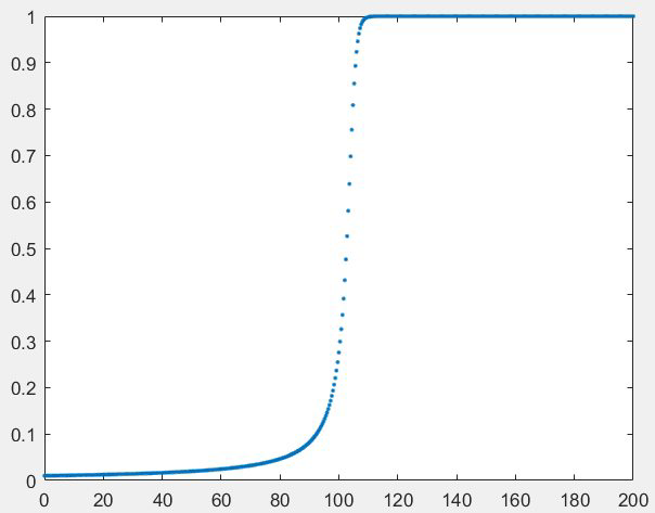图中在中点的位置附近，函数的增长率一下子变得非常快，也就是说在极短的时间内完成了从缓慢增长到稳定状态。那么在这个快速增长的区域，对于数值方法来说是一个很大的挑战，容易出现很大的误差，关于误差这部分我们后面将详述。

作业1：
If the differential equation $\frac{d y}{d t} = f (t)$ only involves $t,$ not $y,$ then its solution is just an integral, $y (t) = \int f (t) d t$ In this situation, the Runge-Kutta method becomes a classic method of numerical quadrature. It should be familiar if you have ever studied such methods. Do you recognize it?

作业2：
What is the solution to $\frac{d y}{d t} = 1 + y^{2}$ with $y (0) = 0$ What happens if you try to use ode4 to solve this equation on the interval $0 \leq t \leq 2$

作业3：
What happens with ode4 if the length of the interval, tfinal-to, is not evenly divisible by the step size, h? For example, if t0=0, tfinal =p i, and h=0 .1. This is one of the hazards of a fixed step size.

作业4：

问：什么是误差阶数？什么是泰勒级数
答：
$o (x^{p})$ 表示的是 $x^{p}$ 的高阶无穷小，也就是当 $p$ 趋近于零时， $o (x^{p})$ 比 $x^{p}$ 更快趋近于零。比如 $x^{2}$ 是 $x$ 的高阶无穷小，可以表示为 $x^{2} = o (x)$ 。回忆一下什么叫作“同阶无穷小”，什么叫作“等价无穷小”(比如 $\sin x$ 和 $x$ )。

将 $f (x)$ 在 $x = a$ 处泰勒展开，得到的是 $f (x) = f (a) + \frac{f^{'} (a)}{1!} (x - a) + \frac{f^{''} (a)}{2!} (x - a)^{2} + \frac{f^{'''} (a)}{3!} (x - a)^{3} + o (x - a)^{3}$

对于欧拉方法ODE1，相当于在 $y_{n}$ 泰勒展开，于是 $y_{n + 1} = y_{n} + \frac{f (t_{n}, y_{n})}{1} h + o (h)$ 注意这里的 $o (h) = m * h^{2}$ ( $m$ 是一个特定常数参见余项形式)。这就说每一步的的误差正比于步长的平方。

对于经典的四阶龙格-库塔法，每一步的local error(局部截断误差，或者说每一步的误差)为 $h^{5}$ 阶，总的global error为 $h^{4}$ 阶，如果让步长减半为 $\frac{h}{2}$ ，那么误差将会减少 $2^{4}$ 。对于ODE1欧拉方法是一个一阶方法，意味着其局部截断误差（每步误差）正比于步长的平方，并且其全局截断误差正比于步长。

命名：odepq uses methods of order p and q

作业：
Modify order x to do further experiments involving the order of our ODE solvers.

ODE23(估计误差，自动调整步长)

问：什么是modern numercial method？
答：
modern numercial method 不同于前面的ODE1欧拉方法或者四阶龙格-库塔方法，它的特点是：
(1) Error estimate and step size control;
(2) Fully accurate continuous interpolant(插值)

也就是不指定步长，而是指定你所需要的精度，程序根据所要求的误差自动调整步长。

Bogacki-Shampine Order 3(2) (ODE23的basis) $\begin{aligned} s_{1} & = f (t_{n}, y_{n}) \\ s_{2} & = f (t_{n} + \frac{h}{2}, y_{n} + \frac{h}{2} s_{1}) \\ s_{3} & = f (t_{n} + \frac{3}{4} h, y_{n} + \frac{3}{4} h s_{2}) \\ t_{n + 1} & = t_{n} + h \\ y_{n + 1} & = y_{n} + \frac{h}{9} (2 s_{1} + 3 s_{2} + 4 s_{3}) \\ s_{4} & = f (t_{n + 1}, y_{n + 1}) \\ e_{n + 1} & = \frac{h}{72} (- 5 s_{1} + 6 s_{2} + 8 s_{3} - 9 s_{4}) \end{aligned}$ 每一步计算的误差都去和这里的 $e_{n + 1}$ 进行比较，如果实际误差比它大，那么减小步长(多插入点)。

先展示ODE23的代码(automatic step choice of ODE23)

function [tout,yout] = ode23tx(F,tspan,y0,arg4,varargin)
%ODE23TX  Solve non-stiff differential equations.  Textbook version of ODE23.
%
%   ODE23TX(F,TSPAN,Y0) with TSPAN = [T0 TFINAL] integrates the system
%   of differential equations dy/dt = f(t,y) from t = T0 to t = TFINAL.
%   The initial condition is y(T0) = Y0.
%
%   The first argument, F, is a function handle or an anonymous function
%   that defines f(t,y).  This function must have two input arguments,
%   t and y, and must return a column vector of the derivatives, dy/dt.
%
%   With two output arguments, [T,Y] = ODE23TX(...) returns a column 
%   vector T and an array Y where Y(:,k) is the solution at T(k).
%
%   With no output arguments, ODE23TX plots the emerging solution.
%
%   ODE23TX(F,TSPAN,Y0,RTOL) uses the relative error tolerance RTOL
%   instead of the default 1.e-3.
%
%   ODE23TX(F,TSPAN,Y0,OPTS) where OPTS = ODESET('reltol',RTOL, ...
%   'abstol',ATOL,'outputfcn',@PLOTFUN) uses relative error RTOL instead
%   of 1.e-3, absolute error ATOL instead of 1.e-6, and calls PLOTFUN
%   instead of ODEPLOT after each successful step.
%
%   More than four input arguments, ODE23TX(F,TSPAN,Y0,RTOL,P1,P2,...),
%   are passed on to F, F(T,Y,P1,P2,...).
%
%   ODE23TX uses the Runge-Kutta (2,3) method of Bogacki and Shampine (BS23).
%
%   Example    
%      tspan = [0 2*pi];
%      y0 = [1 0]';
%      F = @(t,y) [0 1; -1 0]*y;
%      ode23tx(F,tspan,y0);
%
%   See also ODE23.

%   Copyright 2012 - 2015 The MathWorks, Inc.

% Initialize variables.

rtol = 1.e-3;
atol = 1.e-6;
plotfun = @odeplot;
if nargin >= 4 & isnumeric(arg4)
   rtol = arg4;
elseif nargin >= 4 & isstruct(arg4)
   if ~isempty(arg4.RelTol), rtol = arg4.RelTol; end
   if ~isempty(arg4.AbsTol), atol = arg4.AbsTol; end
   if ~isempty(arg4.OutputFcn), plotfun = arg4.OutputFcn; end
end
t0 = tspan(1);
tfinal = tspan(2);
tdir = sign(tfinal - t0);
plotit = (nargout == 0);
threshold = atol / rtol;
hmax = abs(0.1*(tfinal-t0));
t = t0;
y = y0(:);

% Initialize output.

if plotit
   plotfun(tspan,y,'init');
else
   tout = t;
   yout = y.';
end

% Compute initial step size.

s1 = F(t, y, varargin{:});
r = norm(s1./max(abs(y),threshold),inf) + realmin;
h = tdir*0.8*rtol^(1/3)/r;

% The main loop.

while t ~= tfinal
  
   hmin = 16*eps*abs(t);
   if abs(h) > hmax, h = tdir*hmax; end
   if abs(h) < hmin, h = tdir*hmin; end
   
   % Stretch the step if t is close to tfinal.

   if 1.1*abs(h) >= abs(tfinal - t)
      h = tfinal - t;
   end
   
   % Attempt a step.

   s2 = F(t+h/2, y+h/2*s1, varargin{:});
   s3 = F(t+3*h/4, y+3*h/4*s2, varargin{:});
   tnew = t + h;
   ynew = y + h*(2*s1 + 3*s2 + 4*s3)/9;
   s4 = F(tnew, ynew, varargin{:});
      
   % Estimate the error.

   e = h*(-5*s1 + 6*s2 + 8*s3 - 9*s4)/72;
   err = norm(e./max(max(abs(y),abs(ynew)),threshold),inf) + realmin;
      
   % Accept the solution if the estimated error is less than the tolerance.

   if err <= rtol
      t = tnew;
      y = ynew;
      if plotit
         if plotfun(t,y,'');
            break
         end
      else
         tout(end+1,1) = t;
         yout(end+1,:) = y.';
      end
      s1 = s4;     % Reuse final function value to start new step.
   end
   
   % Compute a new step size.

   h = h*min(5,0.8*(rtol/err)^(1/3));
 
   % Exit early if step size is too small.
   
   if abs(h) <= hmin
      warning('Step size %e too small at t = %e.\n',h,t);
      t = tfinal;
   end
end

if plotit
   plotfun([],[],'done');
end

例子1：
F=@(t,y)y; %微分方程，导函数等于函数值本身(其实是指数函数)
ode23(F,[0 1],1) % interval from 0 to 1, 初始值为1，没有output argument(输出参数)

结果为

例子2：
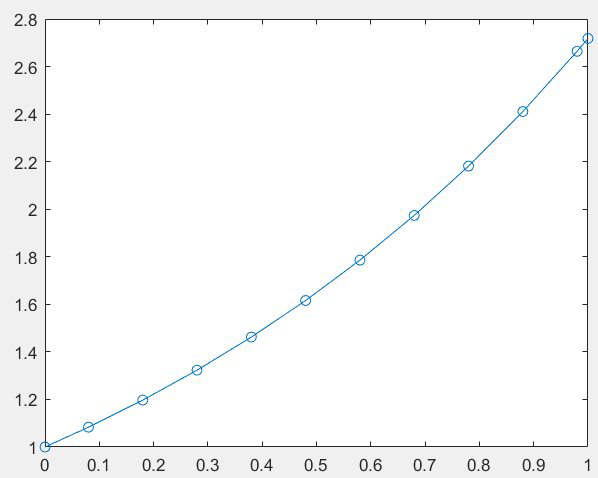
F=@(t,y)y;
[t,y]=ode23(F,[0 1],1) %对比上一个例子加入输出参数
plot(t,y,'o-') %的到的图和上面一样

注意，从0开始第一步选择的步长为0.08(自动调整，满足误差要求)，后面的步长都是0.1，然后最后一步的步长为0.02正好到1。程序的默认误差(default error)为 $10^{- 3}$ 。

例子3：
代码

a=0.25;
y0=15.9;
F=@(t,y)2*(a-t)*y^2
[t,y]=ode23(F,[0 1],y0)
plot(t,y,'-',t,y,'.','markersize',24)

图像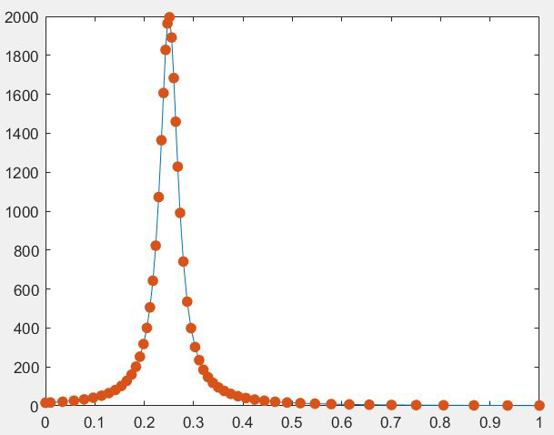图像在0.25附近快速增长，然后又快速下降，这部分是容易出现误差较大的情况，所以ODE23程序自动调整了这一部分的步长，所以点从横轴来看比较密(步长小)，从0.5到1这一部分由于函数值本身变化很小，所以可以在取较大步长的情况下满足默认的误差范围。

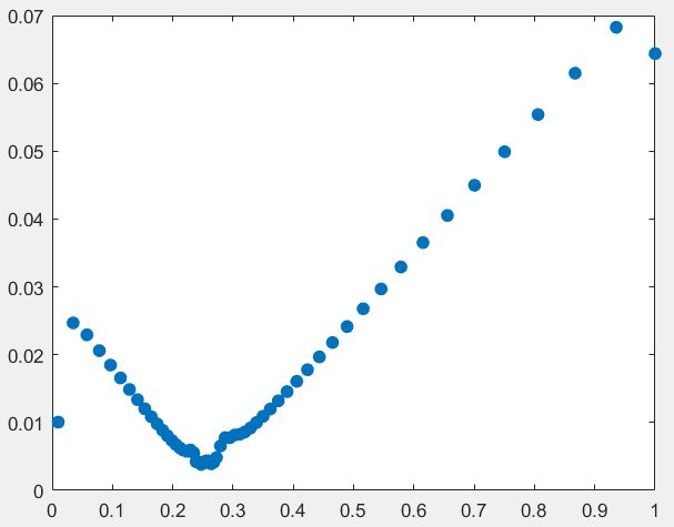
如果根据每一步的步长大小作图，即添加
h=diff(t);
plot(t(2:end),h,'.','markersize',24)这两行代码，可以得到如下图像

问：简单介绍一下各种插值法？
答：

欧拉方法ODE1

中间点法ODE2

经典龙格-库塔法ODE4

ODE23(估计误差，自动调整步长)

You Might Also Like

线性代数-3

MIT-离散随机过程

数学动力学模型-生物

Leave a Reply Cancel reply