课程:
- Probabilistic Systems Analysis and Applied Probability-MIT 配套教材
Introduction to Probability-MIT [mathjax] Discrete Stochastic Processes-MIT
- Statistical Methods in Bioinformatics-UCSD
图谱:Univariate Distribution Relationships
Simulation:
其他资料
基本概念
Probability Models and Axioms
axiom [ˈæksiəm] 公理;格言;自明之理
granularity [ˌɡrænjəˈlærəti] n. 间隔尺寸,[岩] 粒度 the quality of being composed of relatively large particles、
dice [daɪs] 骰子,其复数为die
disjoint 不连贯的;(两个集合)不相交的
Causal Inference 因果推论
【Sample space】(样本空间) \(\Omega\):“List” (set) of possible outcomes. List must be: (1) Mutually exclusive (互相排斥的) (2) Collectively exhaustive (完全穷尽)
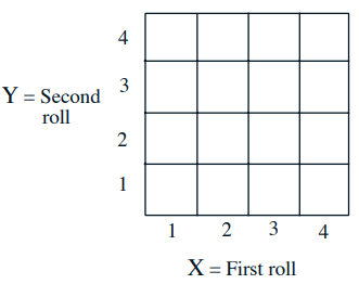
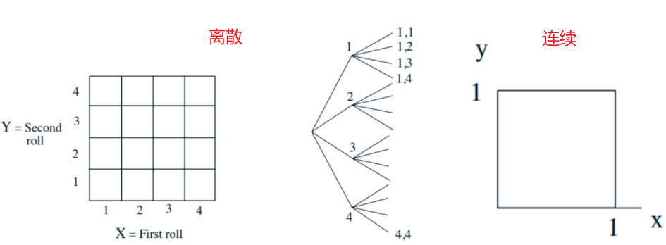 离散样本空间的例子:Two rolls of a tetrahedral die (- Sample space vs. sequential description)
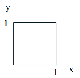
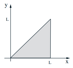
连续样本空间的例子:\(\Omega=\{(x, y) \mid 0 \leq x, y \leq 1\} \)
Probability Axioms:
(1) Nonnegativity: \(\mathbf{P}(A) \geq 0\)
(2) Normalization: \(\mathbf{P}(\Omega)=1\)
(3) Additivity: \(A \cap B=\varnothing\), then \(\mathbf{P}(A \cup B)=\mathbf{P}(A)+\mathbf{P}(B)\)
 Probability law-1: 有限的样本空间
Let every possible outcome have probability 1/16. For the given restrictive condition, we can calculate the corresponding probabilities. Let all outcomes be equally likely. Then $$\mathbf{P}(A)=\frac{\text { number of elements of } A}{\text { total number of sample points }}$$Computing probabilities ≡ counting
Defines fair coins (公平硬币), fair dice (公平骰子), well-shuffled decks (洗好的牌)
 Probability law-2: 无限的样本空间
Two “random” numbers in [0, 1]. Uniform law: Probability = Area
Q1: \( \mathbf{P}(X+Y \leq 1 / 2)=?\)
Q2: \(\mathbf{P}((X, Y)=(0.5,0.3))=?\)
 Probability law-3: 可计数的无限样本空间
Sample space: {1, 2,...}, We are given \(\mathbf{P}(n)=2^{-n}, n=1,2, \ldots\), Find \( \mathbf{P}\)(outcome is even) (Countable additivity axiom)
\( \mathbf{P}(\{2,4,6, \ldots\})=\mathbf{P}(2)+\mathbf{P}(4)+\cdots=\displaystyle\frac{1}{2^{2}}+\frac{1}{2^{4}}+\frac{1}{2^{6}}+\cdots=\frac{1}{3}\)
Independence (Pairwise independence and Mutual exclusivity)
Multiplication rule: $$ \mathbf{P}(A \cap B)=\mathbf{P}(B) \cdot \mathbf{P}(A \mid B)=\mathbf{P}(A) \cdot \mathbf{P}(B \mid A) $$Total probability theorem:$$ \mathbf{P}(B)=\mathbf{P}(A) \mathbf{P}(B \mid A)+\mathbf{P}\left(A^c\right) \mathbf{P}\left(B \mid A^c\right) $$Bayes rule: $$ \mathbf{P}\left(A_i \mid B\right)=\frac{\mathbf{P}\left(A_i\right) \mathbf{P}\left(B \mid A_i\right)}{\mathbf{P}(B)} $$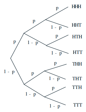 条件概率的例子 :3 tosses of a biased coin: \(\mathbf{P}(H)=p, \mathbf{P}(T)=1-p\)求解
\(\mathbf{P}(T H T)=\)
\( \mathbf{P}(1 \text { head })=\)
\(\mathbf{P}(\text { first toss is } H \mid 1 \text { head })=\)
两个事件独立:\(\mathbf{P}(B \mid A)=\mathbf{P}(B)\),也就是说occurrence of A provides no information about B’s occurrence。如果两个事件独立,那么\(\mathbf{P}(A \cap B)=\mathbf{P}(A) \cdot \mathbf{P}(B \mid A)\)可以改写为$$\mathbf{P}(A \cap B)=\mathbf{P}(A) \cdot \mathbf{P}(B)$$注意上式中的Symmetric with respect to A and B,另外即使\( \mathbf{P}(A)=0\),上式也成立。
独立和互斥
- 【独立性】(Independence)指的是两个变量A和B的发生概率一点关系都没有,更直接的办法是满足\(\mathbf{P}(B \mid A)=\mathbf{P}(B)\)的就说两个事件独立。老王周末有20%概率吃川菜,80%概率喝可乐,他一边吃川菜一边喝可乐概率是3%,吃川菜和和可乐是互相不影响的独立事件吗?
20% X 80% = 16% ≠ 3%
可能川菜太辣,老王改喝酸奶,或者老王喜欢搭配啤酒,这两件事情互相有影响。
如果他一边吃川菜一边喝可乐概率是16%,这两件事就是独立事件,喝可乐不影响吃辣,吃川菜不影响买可乐。 - A和B的发生概率一点关系都没有,这是从结果上来说的,并不代表A的发生对B没有影响,只是说这种可能存在的影响并不会体现在最终的概率计算j结果上。
- A和B相互独立,\(\mathbf{P}(B \mid A)\)和\(\mathbf{P}(B)\)虽然相等,但是注意这是两个不同的样本空间(两个不同的事件),\(\mathbf{P}(B \mid A)\)相当于对\(\mathbf{P}(B)\)的分子分母进行了等比例的约束(缩放)。从笛卡尔积的角度看,如果扑克牌不包含大小王的话,每一张牌是通过有序对来确定(大小 + 花色),随机抽取一张牌,那么抽出特定大小的牌与抽出特定花色的牌显然是两个相互独立的事件,但是如果已知抽中的是♠,那么那是5的概率还是和没有前置条件的结果一样,但是显然其样本空间缩小到原来的四分之一。
 两两独立(pairwise independence)的事件不一定相互独立
-
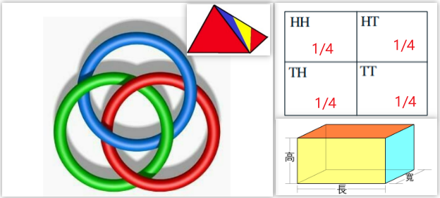
- 波罗梅奥环(Borromean Rings), 三个环两两独立,但三个环无法分离。
- 要造一个体积是V的长方体,长宽高两两独立,但是比如长宽固定了,高就也确定了。
- 投两个骰子,事件A:第一个骰子点数为奇数;事件B:第二个骰子点数为奇数;事件C:两个骰子点数之和为奇数。
于是有\( P(A)=P(B)=P(C) = 1/2 \),\( P(AB)=P(BC)=P(AC) = 1/4 \),\( P(ABC) = 0\)
或者等价的例子(后续会有讨论),投两次骰子,事件A:第一次是H(Head)正面朝上,事件B:第二次是T(Tail)反面朝上,事件C:两次结果一样。 - 一个正四面体的四个面分别有红、黄、蓝、红黄蓝四种颜色,现投此正四面体,记事件A:四面体地面出现红色;事件B:四面体地面出现黄色;事件C:四面体地面出现蓝色。
则\( P(A)=P(B)=P(C) = 1/2 \),\( P(AB)=P(BC)=P(AC) = 1/4 \),\( P(ABC) =1/4\)
-
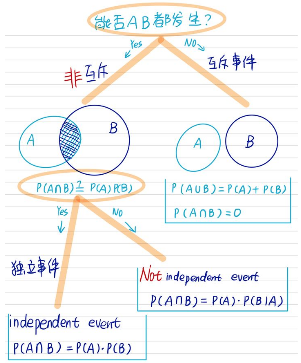
- 【互斥】(Mutual exclusivity):能否AB都发生,我有一只宠物,既是猫又是狗。不可能,这是互斥事件。
参考:
(1) 怎么理解相互独立事件?真的是没有任何关系的事件吗?
(2) 为什么两两独立的事件不一定相互独立?
(3) 怎么理解互斥事件和相互独立事件?
(4) 为什么随机变量X和Y不相关却不一定独立?
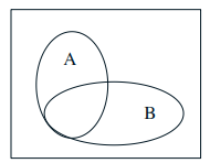
条件可能影响独立(Conditioning may affect independence)
 Conditional independence, given \(C\), is defined as independence under probability law \(\mathbf{P}(\cdot \mid C)\). Assume \(A\) and \(B\) are independent. If we are told that \(C\) occurred, are \(A\) and \(B\) independent? 显然,此时,A和B是disjoint,那么就是属于互斥事件了。从中得到的结论是:Having independence in the original model does not imply independence in a conditional model.
 例子:Two unfair coins, \(A\) and \(B\): \( \mathbf{P}(H \mid \operatorname{coin} A)=0.9, \mathbf{P}(H \mid \operatorname{coin} B)=0.1\). Choose either coin with equal probability.
(1) Once we know it is coin \(A\), are tosses independent? Yes,无论选coin A(上面一个submodel)还是B(下面一个submodel),第一次投出的结果和第二次的没有相互影响概率。
(2) If we do not know which coin it is, are tosses independent? Compare:
(a) \(\mathbf{P}(\text { toss } 11=H)=0.5\times 0.9 + 0.5\times 0.1 = 0.5\)
(b) \(\mathbf{P}(\text { toss } 11=H \mid \text { first } 10 \text { tosses are heads) }\approx 0.9\)
因此前置信息会影响which coin I'm dealing with,显然是用coin A的概率远大于用coin B。
Independence of a collection of events
(1) Intuitive definition: Information on some of the events tells us nothing about probabilities related to the remaining events$$\mathbf{P}\left(A_{1} \cap\left(A_{2}^{c} \cup A_{3}\right) \mid A_{5} \cap A_{6}^{c}\right)=\mathbf{P}\left(A_{1} \cap\left(A_{2}^{c} \cup A_{3}\right)\right)$$(2) Mathematical definition: A collection of events \(A_1, A_2, \ldots, A_n\) are called independent if: $$\mathbf{P}\left(A_{i} \cap A_{j} \cap \cdots \cap A_{q}\right)=\mathbf{P}\left(A_{i}\right) \mathbf{P}\left(A_{j}\right) \cdots \mathbf{P}\left(A_{q}\right)$$for any distinct indices \(\mathrm{I}=i, j, \ldots, q\) (chosen from \(\{1, \ldots, n\}\) )
 串联/并联和可靠性(Reliability):\( p_{i}\): probability that unit \(i\) is "up".如果都是independent units。那么probability that system is "up"?
其他概念
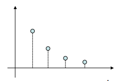
【Probability mass function】(概率质量函数,PMF)描述的是离散随机变量在特定取值上(事件发生)的概率。所有不同事件发生的概率和为1。概率质量函数用\(P(X=k)\)来表示。
【Probability density function】(概率密度函数,PDF)描述的是连续随机变量的概率分布。某一点的概率密度函数是不能表示该事件发生的概率,因为肯定是无穷小,只有概率密度函数在连续随机变量的一段区间上积分,积分的面积才是发生的概率,那么概率密度函数对连续随机变量总的积分面积就是1。概率密度函数一般用\(f(x,\lambda)\),其中\(\lambda\)为数学期望,计算的时候,这个期望是已知的固定值。
【Cumulative Distribution Function】(累积分布函数,CDF)$$ F_{X}(x)=\mathrm{P}(X \leq x)=\int_{-\infty}^{x} f_{X}(t) d t $$
伯努利分布、二项分布、几何分布、帕斯卡分布。
Conditioning and Bayes' Rule
 Conditional probability: \( \mathbf{P}(A \mid B)\) = probability of \(A\), given that \(B\) occurred. \(B\) is our new universe.
Definition: Assuming \( \mathbf{P}(B) \neq 0\)$$\mathbf{P}(A \mid B)=\frac{\mathbf{P}(A \cap B)}{\mathbf{P}(B)}$$
Models based on conditional Multiplication rule probabilities
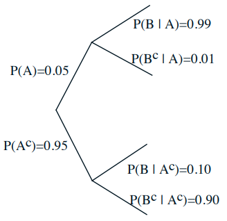 Event A: Airplane is flying above
Event B: Something registers on radar screen
(1) 如果已知事件B发生,那么事件A发生的概率是多少?
(2) 如果已知事件B没有发生,那么事件B发生的概率是多少?
这里其实类似核酸测试,有【灵敏度】,也有【特异性】。如果是一个理想的完美雷达,那么灵敏度和特异性都是100 %。
Multiplication Rule $$\mathbf{P}(A \cap B \cap C)=\mathbf{P}(A) \cdot \mathbf{P}(B \mid A) \cdot \mathbf{P}(C \mid A \cap B)$$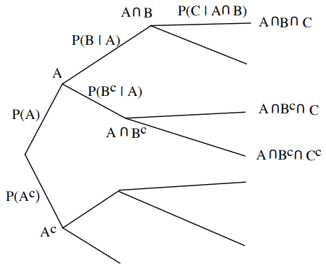
Total probability theorem
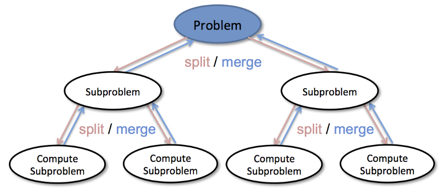
- 【Divide and conquer】(分治法) The divide and conquer approach as the name suggests divides the given problem in parts and then each problem is solved independently.字面上的解释是“分而治之”,就是把一个复杂的问题分成两个或更多的相同或相似的子问题,直到最后子问题可以简单的直接求解,原问题的解即子问题的解的合并。这个技巧是很多高效算法的基础,如排序算法(归并排序、快速排序)、傅立叶变换(快速傅立叶变换)。下图来自Divide and Conquer Algorithm
- Partition of sample space into A1, A2, A3
- Have \(\mathbf{P}\left(B \mid A_{i}\right)\) for every \( i\)
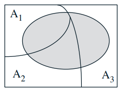
- One way of computing \( \mathbf{P}(B)\): $$ \mathbf{P}(B)=\mathbf{P}\left(A_1\right) \mathbf{P}\left(B \mid A_1\right)+\mathbf{P}\left(A_2\right) \mathbf{P}\left(B \mid A_2\right)+\mathbf{P}\left(A_3\right) \mathbf{P}\left(B \mid A_3\right) $$
Bayes’ rule
- “Prior” probabilities \(\mathbf{P}\left(A_{i}\right)\) (initial “beliefs”)
- We know \(\mathbf{P}\left(B \mid A_{i}\right)\) for each \(i\)
- Wish to compute \(\mathbf{P}\left(A_{i} \mid B\right)\) (revise “beliefs”, given that B occurred)
$$\begin{aligned} \mathrm{P}\left(A_{i} \mid B\right) &=\frac{\mathbf{P}\left(A_{i} \cap B\right)}{\mathbf{P}(B)} \\ &=\frac{\mathbf{P}\left(A_{i}\right) \mathbf{P}\left(B \mid A_{i}\right)}{\mathbf{P}(B)} \\ &=\frac{\mathbf{P}\left(A_{i}\right) \mathbf{P}\left(B \mid A_{i}\right)}{\sum_{j} \mathbf{P}\left(A_{j}\right) \mathbf{P}\left(B \mid A_{j}\right)} \end{aligned}$$
贝叶斯定理中文简介和实例
简单的情况,贝叶斯定理是关于随机事件A和B的条件概率的一则定理$$P(A | B)=\displaystyle\frac{P(B | A) P(A)}{P(B)}$$总而言之,就是A,B两件事情不是完全独立的,两者之间存在相互联系。比如每4个人中就有一个人因为心脏病而死亡,也就是说是四分之一的概率,那么哥哥和弟弟同时因为心脏病而死亡的概率不是简单的十六分之一,因为如果哥哥因为心脏病而死亡,那么弟弟由于和哥哥基因以及生活方式的相似性,得心脏病的几率要比原来的四分之一高很多。问题的关键是A和B之间存在correlation。
注:A和B相互独立,则有\(\mathbf{P}(B \mid A)\)和\(\mathbf{P}(B)\)。
例子-1:抽红球和蓝球(李永乐视频):有三个完全相同的盒子,有一个盒子装了两个红球RR,一个盒子里装了两个蓝球BB,一个盒子里装了一个红球一个蓝球RB,现在有一个同学随机摸了一个球发现是红球,那么该盒子里另一个球也是红球的概率是多少?
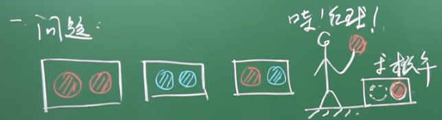 (1) 先采用列举法,摸出红球有三种可能,而且是等可能的;摸出一个红球,盒子里另外一个球也是红球占两种可能。所以最终的结果就是这两个数相处,得到2/3。
(2) 采用条件概率(贝叶斯公式)
事件A:第一个球摸出的是红球,概率为\( P(A)=\displaystyle\frac{1}{3}+\frac{1}{3} \times \displaystyle\frac{1}{2}=\displaystyle\frac{1}{2}\)
事件B:摸到两个红球(同一个盒子里),显然概率就是\(P(B)=\displaystyle\frac { 1 }{ 3 } \)
显然 AB = B,因此\( P(B \mid A)=\displaystyle\frac{P(A B)}{P(A)}=\displaystyle\frac { 1/3 }{1/2 } =\displaystyle\frac {2 }{3 } \)
 例子-2:国王的兄弟姐妹(The king’s sibling) The king comes from a family of two children. What is the probability that his sibling is female?
这里面存在的问题是too loosely stated,所以我们必须在开始计算前做一些假设,boys have precedence。即使一男一女,女儿先出生,也是儿子享有继承王位的权利。另外假设生孩子的时候,生男生女的概率都是50 %,而且生男生女之间相互独立independent。更复杂的情形可以参考MIT-网站视频
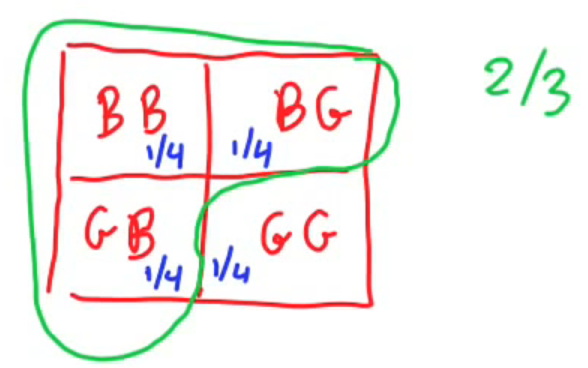
例子-3:一个家庭里面有两个孩子,其中之一是女孩儿,求另一个也是女孩儿的概率?
有人认为答案是1/2,因为生男生女没有差异,概率都是1/2,有人认为答案是1/3。关键在于对这句话“其中之一是女孩儿”的理解,有两种理解方式:
(1) 至少有一个是女孩儿
(2) A是女孩儿
所有可能的情况是A男B男,A女B女,A男B女,A女B男。如果采用第一种理解方式,那么答案就是1/3;如果采用第二种理解方式就是1/2。按照题意,出题者想说的是第一种的理解方式。
例子-4: 三个囚犯问题,有A、B、C三个囚犯第二天要被处决了,但是突然来了一个消息说他们其中一个人被赦免了。看守知道谁被赦免了,但是看守不能告诉任何一个人到底谁被赦免了,比如不能告诉A你被赦免了或者被杀死了,但是可以告诉A你的小伙伴B(或者C)要被处决。如果告诉A你的小伙伴B被赦免了,等于告诉A你要被杀死,这是不允许的。另外看守也不说假话。
现在A去问看守,看守说B要被杀死了,此时A很高兴,因为他觉得自己的被赦免的概率从1/3变为1/2。看守说不是的,你被赦免的概率依然是1/3,而C被赦免的概率是2/3。到底谁说得对?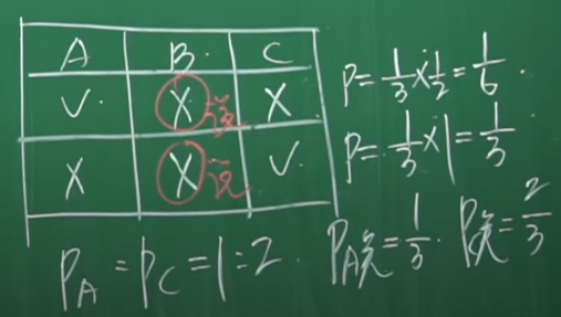
讨论:有人问,看守告诉A你的小伙伴B被杀死的时候,A和C的地位不是一样的吗?为什么A赦免的概率比C小呢?那是因为当A去问看守的时候,A和C的地位就不等同了,A去问看守,看守就不会告诉A你被杀死还是赦免,只会在B和C中选一个。
例子-3和4,来自李永乐视频,例子-4也可以看知乎更详细的分析有趣的数学——违反直觉的囚犯问题
例子-5: 三门问题,在美国的一档节目Let's Make a Deal 中,主持人蒙提·霍尔设置了一项小游戏:在你的面前有三扇门,其中一扇背后藏有一辆价值不菲的汽车;剩下的两扇背后则分别是两头山羊。你现在有机会选择一扇门,选好之后先不要打开,这时主持人会在另外两扇门中,开启一扇山羊门。现在你有两个选择,是应该维持原来的选择,还是转而选择另一扇没有开启的门?
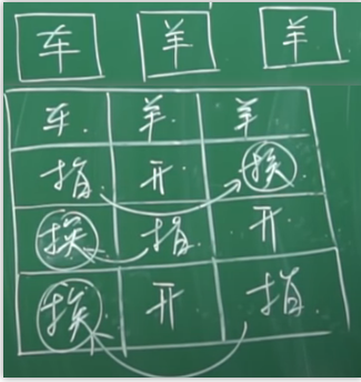 不改变决策,抽中汽车的概率是1/3;
改变决策,抽中汽车的概率是2/3。
参考李永乐视频,三门问题:直觉究竟去了哪里?-返朴
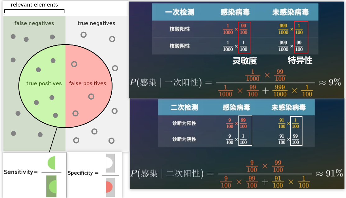
例子-6:核酸检测准不准,核酸阴性就一定表示自己没有被感染吗?核酸阳性就一定表示自己被感染了吗?
如果一个人感染了,那么检测结果可能是真阳性,或者假阴性;如果一个人没有被感染,那么检测结果可能就是真阴性,或者假阳性。
灵敏度 = 真阳性 / (真阳性 + 假阴性) 其实就是给你一堆都感染的人,实际测出阳性的比例。
特异性 = 真阴性 / (真阴性 + 假阳性) 其实就是给你一堆都没有被感染的人,实际测出阴性的比例。
现在假设一个国家有千分之一的人感染了新冠病毒,然后进行核酸检测,其灵敏度和特异性都是99/100,现在张三第一次检测是阳性,那么张三真实感染的概率有多大?
Discrete Random Variables
Counting
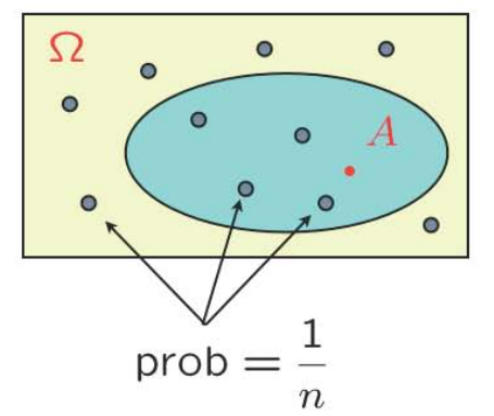 离散均匀分布:Let all sample points be equally likely. Then, $$\mathbf{P}(A)=\displaystyle\frac{\text { number of elements of } A}{\text { total number of sample points }}=\frac{|A|}{|\Omega|}$$Just count...
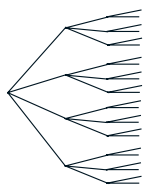 Basic counting principle:总共做\(r\)次选择,其中第\(i\)次选择的内容为\( n_{i}\),那么Number of choices is: \( n_{1} n_{2} \cdots n_{r}\)。下面举四个例子:
(1) 假设Number of license plates (车辆牌照) with 3 letters and 4 digits,那么总共有26*26*26*10*10*10*10种可能的情况。如果if repetition is prohibited,那么总共有26*25*24*10*9*8*7可能的情况。
(2) Number of ways of ordering \(n\) elements is: \(n!\)
(3) Number of subsets of \(\{1, \ldots, n\}= 2^n\)
(4) Probability that six rolls of a six-sided die all give different numbers?
答:Number of outcomes that make the event happen: \(6 !\);样本空间元素的数量为\(6^{6}\)。因此概率为\(\displaystyle\frac{|A|}{|\Omega |}=\displaystyle\frac{6!}{6^{6}}\)。
Combinations
\( \left(\begin{array}{l} n \\ k \end{array}\right)\): number of \(k\)-element subsets of a given \(n\)-element set
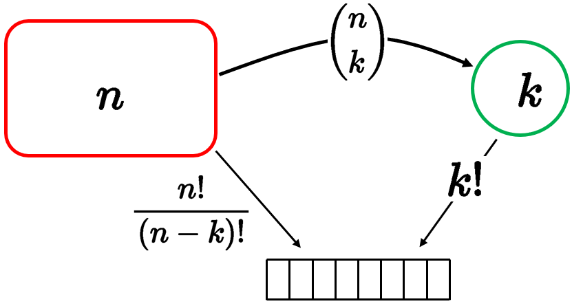 Two ways of constructing an ordered sequence of \(k \) distinct items:
方法1:Choose the \(k\) items one at a time:
\(n(n-1) \cdots(n-k+1)=\displaystyle\frac{n !}{(n-k) !}\) choices
方法2:Choose \(k\) items \(\left(\begin{array}{l}n \\ k\end{array}\right)\), then order them (\(k !\) possible orders).
殊途同归,于是有$$ \left(\begin{array}{c} n \\ k \end{array}\right) \cdot k !=\frac{n !}{(n-k) !} $$\(\left(\begin{array}{l}n \\ k\end{array}\right)=\displaystyle\frac{n !}{k !(n-k) !}\)其实就是Binomial Coefficients (二项式系数),而且\(\displaystyle\sum_{k=0}^n\left(\begin{array}{l}n \\ k\end{array}\right)=2^n\)就是total number of subsets,其实就是\(2^n\)。
Binomial probabilities 二项(分布)概率
\( n\) independent coin tosses, \( \mathbf{P}(H)=p\). 求解\(\mathbf{P}(H T T H H H)\)的方法为:\( \mathbf{P}(\text { sequence })=p^{\# \text { heads }}(1-p)^{\# \text { tails }}\)。对于\(n\)次试验,出现\(k\)次正面朝上的概率,而且不要求sequence$$ \mathbf{P}(k \text { heads })=\sum_{k-\text { head seq. }} \mathbf{P}(\text { seq. })=(\# \text { of } k-\text { head seqs. }) \cdot p^k(1-p)^{n-k}=\left(\begin{array}{l} n \\ k \end{array}\right) p^k(1-p)^{n-k} $$
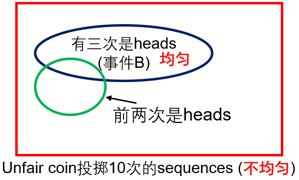 掷硬币问题:Event \( B\): 3 out of 10 tosses were “heads”. Given that \( B\) occurred, what is the (conditional) probability that the first 2 tosses were heads?
答:All outcomes in set \( B\) are equally likely: probability \( p^{3}(1-p)^{7}\),于是Conditional probability law is uniform。其中\(\left(\begin{array}{c}10 \\ 3\end{array}\right)\),其中前两次都是heads有8种可能的情形。于是答案为\( 8/C_3^{10}\)。
Partitions (分区)
52-card deck, dealt to 4 players. Find \(\mathbf{P}\) (each gets an ace,就是牌A)?
分析:Outcome: number of outcomes$$ \begin{aligned} \# \Omega &=\left(\begin{array}{l} 52 \\ 13 \end{array}\right) \cdot\left(\begin{array}{l} 39 \\ 13 \end{array}\right) \cdot\left(\begin{array}{l} 26 \\ 13 \end{array}\right) \cdot\left(\begin{array}{l} 13 \\ 13 \end{array}\right) \\ &=\frac{52 !}{13 !(52-13) !} \cdot \frac{39 !}{13 !(39-13) !} \cdot \frac{26 !}{13 !(26-13) !} \cdot \frac{13 !}{13 !(13-13) !}=\frac{52 !}{13 !^4} \end{aligned} $$Count number of ways of distributing the four aces: \(4 \cdot 3 \cdot 2\) 保证4个人每个人都有一张A。Count number of ways of dealing the remaining \(48\) cards \(\displaystyle\frac{48 !}{12 ! 12 ! 12 ! 12 !}\)。因此最终的答案为\(\displaystyle\frac{4 \cdot 3 \cdot 2 \displaystyle\frac{48 !}{12 ! 12 ! 12 ! 12 !}}{\displaystyle\frac{52 !}{13 ! 13 ! 13 ! 13 !}}\)
PMF和期望
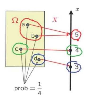
Random variables: An assignment of a value (number) to every possible outcome. Mathematically: A random variable is not random. It's not a variable. It's just a function from the sample space \(\omega \) to the real numbers, discrete or continuous values. 注意可以有多个random variables defined on the same sample space。
 Notation:
— random variable \(X\):function sample space (\omega \) to real numbers
— numerical value \(x\) \(\in \mathbb{R}\)
【Probability mass function 】(PMF)
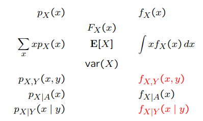
 “probability distribution” of \(X\)$$ p_X(x)=\mathbf{P}(X=x)=\mathbf{P}(\{\omega \in \Omega \text { s.t. } X(\omega)=x\}) $$Properties: \( p_{X}(x) \geq 0 \quad \displaystyle\sum_{x} p_{X}(x)=1\)
例子: Assume independent tosses,不断投骰子,直到正面朝上,这个过程需要的总的投骰子次数为变量\(X\)$$ p_X(k)=\mathbf{P}(X=k)=\mathbf{P}(T T \cdots T H)=(1-p)^{k-1} p, \quad k=1,2, \ldots $$这样的PMF被称【geometric PMF】,\( X\) 被称作geometric random variable。

PMF \( p_{X}(x)\)的计算方法:
(1) collect all possible outcomes for which \( X\) is equal to \( x\)
(2) add their probabilities
(3) repeat for all \(x\)
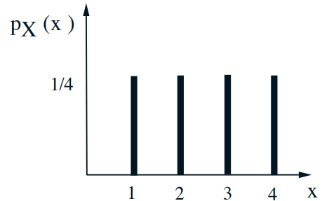
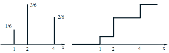
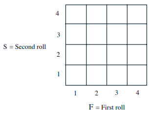 例子:Two independent variables of a fair tetrahedral die:F-outcome of first throw; S-outcome of second throw. 现在要研究的随机变量是X = min(F, S),比如\( p_{X}(2)=5/16\)
【Binomial PMF】
\( X\): number of heads in \( n\) independent coin tosses. \( \mathbf{P}(H)=p\). Let \( n=4\)$$ \begin{aligned} p_X(2) &=\mathbf{P}(H H T T)+\mathbf{P}(H T H T)+\mathbf{P}(H T T H)+\mathbf{P}(T H H T)+\mathbf{P}(T H T H)+\mathbf{P}(T T H H) \\ &=6 p^2(1-p)^2 \\ &=\left(\begin{array}{c} 4 \\ 2 \end{array}\right) p^2(1-p)^2 \end{aligned} $$In general:$$p_{X}(k)=\left(\begin{array}{l} n \\ k \end{array}\right) p^{k}(1-p)^{n-k}, \quad k=0,1, \ldots, n$$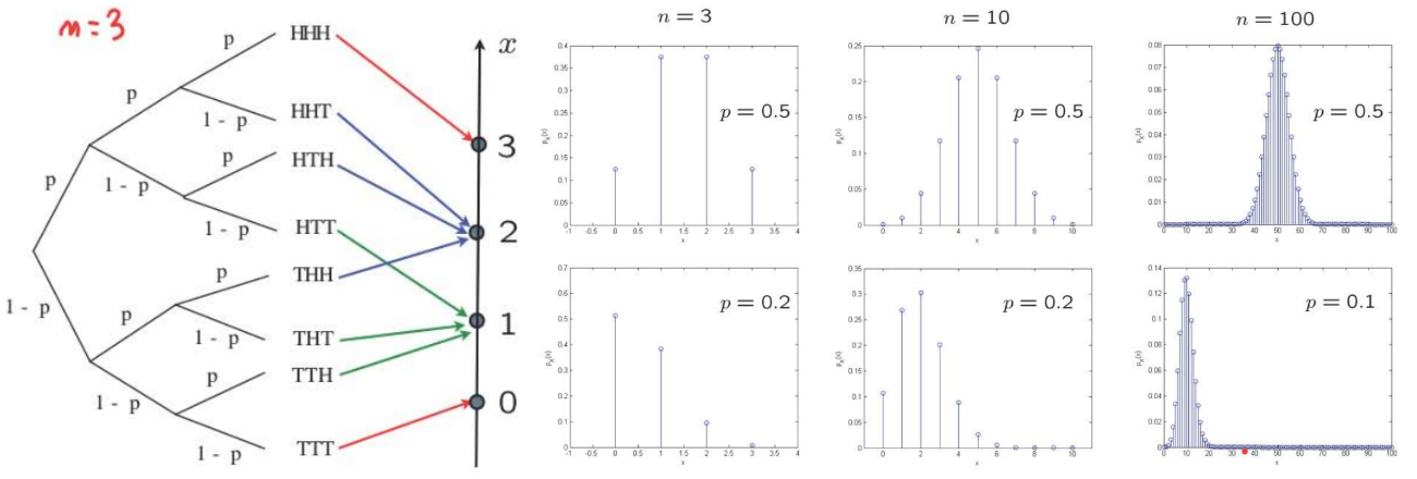
Expectation(期望)$$\mathbf{E}[X]=\sum_{x} x p_{X}(x)$$Interpretations:
– Center of gravity of PMF
– Average in large number of repetitions of the experiment (to be substantiated later in this course)
例子: Uniform on \(0,1, \ldots, n\)
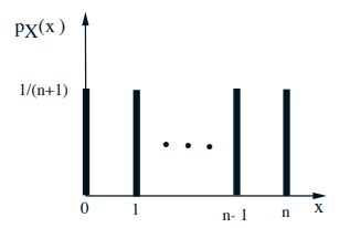 \( \mathrm{E}[X]=0 \times \displaystyle\frac{1}{n+1}+1 \times \displaystyle\frac{1}{n+1}+\cdots+n \times \displaystyle\frac{1}{n+1}=\)
Properties of expectations
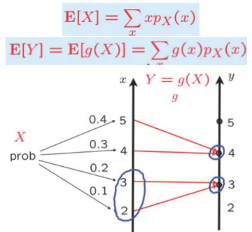
- Let \( X \) be a 实数 and let \( Y = g(X)\)
— Hard: \( \mathbf{E}[Y]=\displaystyle\sum_{y} y p_{Y}(y)\)
— Easy: \( \mathbf{E}[Y]=\displaystyle\sum_{x} g(x) p_{X}(x)\) - Caution: In general, \(\mathbf{E}[g(X)] \neq g(\mathbf{E}[X])\) These two operations of taking averages and taking functions do not commute.
- Properties: If \( \alpha, \beta\) are constants, then: \( \mathbf{E}[\alpha X+\beta]=\alpha \mathbf{E}[X]+\beta\)
Variance(方差)
Recall: \(\mathbf{E}[g(X)]=\displaystyle\sum_{x} g(x) p_{X}(x)\)
Second moment: \( \mathbf{E}\left[X^{2}\right]=\displaystyle\sum_{x} x^{2} p_{X}(x)\)
Variance: average squared distance from the mean下面的推导可以参考这里$$\begin{aligned} \operatorname{var}(X) &=\mathbf{E}\left[(X-\mathbf{E}[X])^{2}\right] \\ &=\sum_{x}(x-\mathbf{E}[X])^{2} p_{X}(x) \\ &=\mathbf{E}\left[X^{2}\right]-(\mathbf{E}[X])^{2} \end{aligned}$$
Standard deviation: \(\sigma_{X}=\sqrt{\operatorname{var}(X)}\)
Properties:
(1) \( \operatorname{var}(X) \geq 0\)
(2) \( \operatorname{var}(\alpha X+\beta)=\alpha^{2} \operatorname{var}(X)\)
Examples and Joint PMFs
Random speed
Traverse a 200 mile distance at constant but random speed \( V\)

- \(d=200, T=t(V)=200 / V\)
- \(E[V]=\displaystyle\frac{1}{2} \cdot 1+\displaystyle\frac{1}{2} \cdot 200=100.5\)
- \(\operatorname{var}(V)=\displaystyle\frac{1}{2}(1-100.5)^{2}+\displaystyle\frac{1}{2}(200-100.5)^{2}\)
- \(\sigma_{V}=\sqrt{100^{2}}=100\)
- \(\mathbf{E}[T]=\mathbf{E}[t(V)]=\sum_{v} t(v) p_{V}(v)=\displaystyle\frac{1}{2} 200+\frac{1}{2} \cdot 1\)
- \(\mathbf{E}[T V]=200 \neq \mathbf{E}[T] \cdot \mathbf{E}[V]\)
- \(\mathbf{E}[200 / V]=\mathbf{E}[T] \neq 200 / \mathbf{E}[V]\)
Conditional PMF and expectation
- \(p_{X \mid A}(x)=\mathbf{P}(X=x \mid A)\) 搞清楚这个概念
- \(\mathbf{E}[X \mid A]=\sum_{x} x p_{X \mid A}(x)\) 搞清楚这个概念
- Let \(A=\{X \geq 2\}\)
-
- \(p_{X \mid A}(x)=1 / 3 \quad x=2,3,4\)
- \(\mathbf{E}[X \mid A]=\displaystyle\frac{1}{3} \cdot2+\displaystyle\frac{1}{3} \cdot 3+\displaystyle\frac{1}{3} \cdot 4\)
-
Geometric PMF
- \(X:\) number of independent coin tosses until first head$$ \begin{gathered} p_{X}(k)=(1-p)^{k-1} p, \quad k=1,2, \ldots \\ \mathbf{E}[X]=\sum_{k=1}^{\infty} k p_{X}(k)=\sum_{k=1}^{\infty} k(1-p)^{k-1} p \end{gathered} $$
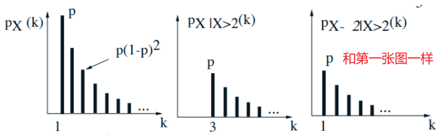
- Memoryless property: Given that \(X>2\), the r.v. \(X-2\) has same geometric PMF
Total Expectation theorem

- Partition of sample space into disjoint events \(A_{1}, A_{2}, \ldots, A_{n}\)$$ \begin{aligned} &\mathbf{P}(B)=\mathbf{P}\left(A_{1}\right) \mathbf{P}\left(B \mid A_{1}\right)+\cdots+\mathbf{P}\left(A_{n}\right) \mathbf{P}\left(B \mid A_{n}\right) \\ &p_{X}(x)=\mathbf{P}\left(A_{1}\right) p_{X \mid A_{1}}(x)+\cdots+\mathbf{P}\left(A_{n}\right) p_{X \mid A_{n}}(x) \\ &\mathrm{E}[X]=\mathbf{P}\left(A_{1}\right) \mathrm{E}\left[X \mid A_{1}\right]+\cdots+\mathbf{P}\left(A_{n}\right) \mathrm{E}\left[X \mid A_{n}\right] \end{aligned} $$
- Geometric example:$$ \begin{array}{l} A_{1}:\{X=1\}, \quad A_{2}:\{X>1\} \\ \mathbf{E}[X]=\mathbf{P}(X=1) \mathbf{E}[X \mid X=1]+\mathbf{P}(X>1) \mathbf{E}[X \mid X>1] \\\quad \quad \, \,= p\cdot 1+(1-p)\cdot (\mathbf{E}[X]+1)\end{array}$$
- 注意最后一步借助了\(\mathbf{E}[X \mid X-1>0])=\mathbf{E}[X-1 \mid X-1>0]+1= \mathbf{E}[X]+1\)
\(\mathbf{E}[X-1 \mid X-1>0]\)表示的是expected value of the remaining coin flips until I obtain heads, given that the first one was tails.
解方程Solve to get 几何分布的期望为 \(\mathbf{E}[X]=1 / p\)
参考:
(1) 几何分布期望,方差推导
(2) 常见概率分布的期望和方差推导
Joint PMFs
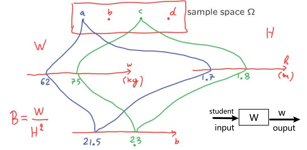
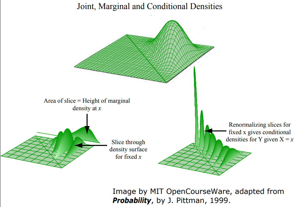
A typical experiment may have several random variables associated with that experiment. A student has height and weight. If I give you the PMF of height, that tells me something about distribution of heights in the class. 同理,PMF of weight. But if I want to ask a question about the association between height and weight. Then I need to know something little more, how height and weight relate to each other. Joint PMFs can give us this.
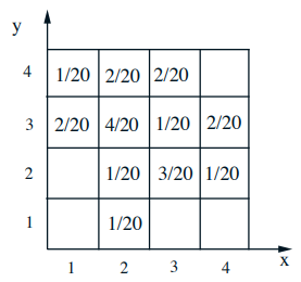
- \(p_{X, Y}(x, y)=\mathbf{P}(X=x\) and \(Y=y)\) 这个就是joint probability (针对两个变量的分布一起研究)
- \(\sum_{x} \sum_{y} p_{X, Y}(x, y)=1\)
- \(p_{X}(x)=\sum_{y} p_{X, Y}(x, y)\) 其实是就是固定\(X\)的值,然后加和每一列,这个就是marginal (针对其中一个变量的分布来研究)
- \(p_{X \mid Y}(x \mid y)=\mathbf{P}(X=x \mid Y=y)=\displaystyle\frac{p_{X, Y}(x, y)}{p_{Y}(y)}\) 固定\(Y=y\),\( X\)在变化
比如选择固定\(Y=2\),那么不同\( x\)的概率分别为0、1/5、3/5、1/5。 - \(\sum_{x} p_{X \mid Y}(x \mid y)=1\)
Multiple Discrete Random Variables
Independent random variables
\(p_{X, Y, Z}(x, y, z)=p_{X}(x) p_{Y \mid X}(y \mid x) p_{Z \mid X, Y}(z \mid x, y)\)
- Random variables \(X, Y, Z\) are independent if: \(p_{X, Y, Z}(x, y, z)=p_{X}(x) \cdot p_{Y}(y) \cdot p_{Z}(z)\) for all \(x, y, z\)

- Independent?
- What if we condition on \(X \leq 2\) and \(Y \geq 3\) ?
Expectations
$$ \begin{gathered} \mathbf{E}[X]=\sum_{x} x p_{X}(x) \\ \mathbf{E}[g(X, Y)]=\sum_{x} \sum_{y} g(x, y) p_{X, Y}(x, y) \end{gathered} $$
- In general: \(\mathbf{E}[g(X, Y)] \neq g(\mathbf{E}[X], \mathbf{E}[Y])\)
- \(\mathbf{E}[\alpha X+\beta]=\alpha \mathbf{E}[X]+\beta\)
- \(\mathbf{E}[X+Y+Z]=\mathbf{E}[X]+\mathbf{E}[Y]+\mathbf{E}[Z]\)
- If \(X, Y\) are independent:
-
- \(\mathbf{E}[X Y]=\mathbf{E}[X] \mathbf{E}[Y]\)
- \(\mathbf{E}[g(X) h(Y)]=\mathbf{E}[g(X)] \cdot \mathbf{E}[h(Y)]\)
-
Variances
- \(\operatorname{Var}(a X)=a^{2} \operatorname{Var}(X)\)
- \(\operatorname{Var}(X+a)=\operatorname{Var}(X)\)
- Let \(Z=X+Y\). If \(X, Y\) are independent:$$\operatorname{Var}(X+Y)=\operatorname{Var}(X)+\operatorname{Var}(Y)$$
- Examples:
-
- If \(X=Y, \operatorname{Var}(X+Y)=\)
- If \(X=-Y, \operatorname{Var}(X+Y)=\)
- If \(X, Y\) indep., and \(Z=X-3 Y\), \(\operatorname{Var}(Z)=\)
-
Binomial mean and variance
- \(X=\#\) of successes in \(n\) independent trials
– probability of success \(p\) $$ E[X]=\sum_{k=0}^{n} k\left(\begin{array}{l} n \\ k \end{array}\right) p^{k}(1-p)^{n-k} $$ - \(X_{i}= \begin{cases}1, & \text { if success in trial } i \\ 0, & \text { otherwise }\end{cases}\)
- \(\mathbf{E}\left[X_{i}\right]=\)
- \(\mathbf{E}[X]=\)
- \(\operatorname{Var}\left(X_{i}\right)=\)
- \(\operatorname{Var}(X)=\)
The hat problem
- \(n\) people throw their hats in a box and then pick one at random.
-
- \(X:\) number of people who get their own hat
- Find \(\mathbf{E}[X]\)$$ X_{i}= \begin{cases}1, & \text { if } i \text { selects own hat } \\ 0, & \text { otherwise. }\end{cases} $$
-
- \(X=X_{1}+X_{2}+\cdots+X_{n}\)
- \(\mathbf{P}\left(X_{i}=1\right)=\)
- \(\mathbf{E}\left[X_{i}\right]=\)
- Are the \(X_{i}\) independent?
- \(\mathbf{E}[X]=\)
Variance in the hat problem
- \(\operatorname{Var}(X)=\mathrm{E}\left[X^{2}\right]-(\mathrm{E}[X])^{2}=\mathbf{E}\left[X^{2}\right]-1\)$$ X^{2}=\sum_{i} X_{i}^{2}+\sum_{i, j: i \neq j} X_{i} X_{j} $$
- \(\mathbf{E}\left[X_{i}^{2}\right]=\)$$ \begin{aligned} \mathbf{P}\left(X_{1} X_{2}=1\right) &=\mathbf{P}\left(X_{1}=1\right) \cdot \mathbf{P}\left(X_{2}=1 \mid X_{1}=1\right) \\ &= \end{aligned} $$
- \(\mathrm{E}\left[X^{2}\right]=\)
- \(\operatorname{Var}(X)=\)
Continuous Random Variables
单变量
A continuous r.v. is described by a probability density function \(f_{X}\)
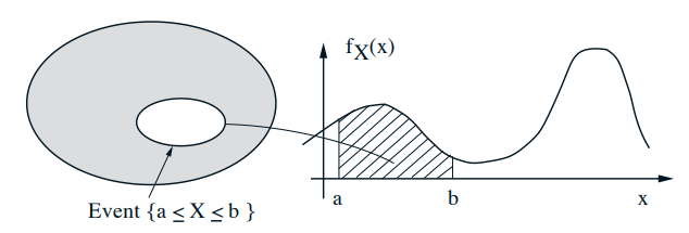 $$ \begin{gathered} \mathbf{P}(a \leq X \leq b)=\int_{a}^{b} f_{X}(x) d x \\ \int_{-\infty}^{\infty} f_{X}(x) d x=1 \\ \mathbf{P}(x \leq X \leq x+\delta)=\int_{x}^{x+\delta} f_{X}(s) d s \approx f_{X}(x) \cdot \delta \\ \mathbf{P}(X \in B)=\int_{B} f_{X}(x) d x, \quad \text { for "nice" sets } B \end{gathered} $$
Means and variances
- \(\mathbf{E}[X]=\displaystyle\int_{-\infty}^{\infty} x f_{X}(x) d x\)
- \(\mathbf{E}[g(X)]=\displaystyle\int_{-\infty}^{\infty} g(x) f_{X}(x) d x\)
- \(\operatorname{var}(X)=\sigma_{X}^{2}=\displaystyle\int_{-\infty}^{\infty}(x-\mathbf{E}[X])^{2} f_{X}(x) d x\)
- Continuous Uniform r.v.
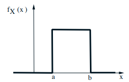
- \(f_{X}(x)=\quad a \leq x \leq b\)
- \(\mathbf{E}[X]=\)
- \(\sigma_{X}^{2}=\displaystyle\int_{a}^{b}\left(x-\displaystyle\frac{a+b}{2}\right)^{2} \frac{1}{b-a} d x=\frac{(b-a)^{2}}{12}\)
Cumulative distribution function (CDF)
$$ F_{X}(x)=\mathrm{P}(X \leq x)=\int_{-\infty}^{x} f_{X}(t) d t $$

- Also for discrete r.v.'s: $$ F_{X}(x)=\mathbf{P}(X \leq x)=\sum_{k \leq x} p_{X}(k) $$
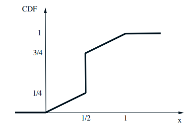
Mixed distributions
- Schematic drawing of a combination of a PDF and a PMF
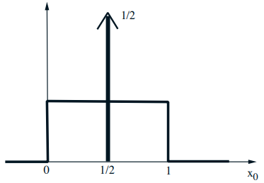
- The corresponding CDF: \(F_{X}(x)=\mathbf{P}(X \leq x)\)
Gaussian (normal) PDF
- Standard normal \(N(0,1): f_{X}(x)=\displaystyle\frac{1}{\sqrt{2 \pi}} e^{-x^{2} / 2}\)

- \(\mathbf{E}[X]=\quad \operatorname{var}(X)=1\)
- General normal \(N\left(\mu, \sigma^{2}\right):\) $$ f_{X}(x)=\frac{1}{\sigma \sqrt{2 \pi}} e^{-(x-\mu)^{2} / 2 \sigma^{2}} $$
- It turns out that: $$ \mathbf{E}[X]=\mu \quad \text { and } \operatorname{Var}(X)=\sigma^{2} $$
- Let \(Y=a X+b\)
-
- Then: \(\mathbf{E}[Y]=\quad \operatorname{Var}(Y)=\)
- Fact: \(Y \sim N\left(a \mu+b, a^{2} \sigma^{2}\right)\)
-
Calculating normal probabilities
- No closed form available for CDF
– but there are tables (for standard normal) - If \(X \sim N\left(\mu, \sigma^{2}\right)\), then \(\displaystyle\frac{X-\mu}{\sigma} \sim N(\) )
- If \(X \sim N(2,16)\)
\(\mathbf{P}(X \leq 3)=\mathbf{P}\left(\displaystyle\frac{X-2}{4} \leq \frac{3-2}{4}\right)=\operatorname{CDF}(0.25)\)
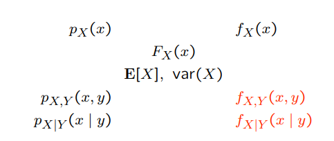
The constellation of concepts
多变量
Summary of concepts
Continuous r.v.'s and pdf 's
 \(\mathbf{P}(a \leq X \leq b)=\displaystyle\int_{a}^{b} f_{X}(x) d x\)
- \(\mathbf{P}(x \leq X \leq x+\delta) \approx f_{X}(x) \cdot \delta\)
- \(\mathrm{E}[g(X)]=\displaystyle\int_{-\infty}^{\infty} g(x) f_{X}(x) d x\)
Joint PDF \(f_{X, Y}(x, y)\)
$$ \mathbf{P}((X, Y) \in S)=\iint_{S} f_{X, Y}(x, y) d x d y $$
- Interpretation: $$ \mathbf{P}(x \leq X \leq x+\delta, y \leq Y \leq y+\delta) \approx f_{X, Y}(x, y) \cdot \delta^{2} $$
- Expectations: $$ \mathbf{E}[g(X, Y)]=\int_{-\infty}^{\infty} \int_{-\infty}^{\infty} g(x, y) f_{X, Y}(x, y) d x d y $$
- From the joint to the marginal: $$ f_{X}(x) \cdot \delta \approx \mathbf{P}(x \leq X \leq x+\delta)= $$
- \(X\) and \(Y\) are called independent if \(f_{X, Y}(x, y)=f_{X}(x) f_{Y}(y)\) for all \(x, y\)
Buffon's needle—多变量例子
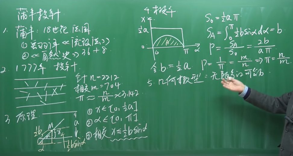
- Parallel lines at distance \(d\) Needle of length \(\ell\) (assume \(\ell<d\) )
- Find \(\mathbf{P}\) (needle intersects one of the lines)
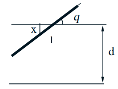
- \(X \in[0, d / 2]:\) distance of needle midpoint to nearest line
- Model: \(X, \Theta\) uniform, independent $$ f_{X, \Theta}(x, \theta)=\quad 0 \leq x \leq d / 2,0 \leq \theta \leq \pi / 2 $$
- Intersect if \(X \leq \frac{\ell}{2} \sin \Theta\) $$ \begin{aligned} \mathbf{P}\left(X \leq \frac{\ell}{2} \sin \Theta\right) &=\iint_{x \leq \frac{\ell}{2} \sin \theta} f_{X}(x) f_{\Theta}(\theta) d x d \theta \\ &=\frac{4}{\pi d} \int_{0}^{\pi / 2} \int_{0}^{(\ell / 2) \sin \theta} d x d \theta \\ &=\frac{4}{\pi d} \int_{0}^{\pi / 2} \frac{\ell}{2} \sin \theta d \theta=\frac{2 \ell}{\pi d} \end{aligned} $$
-
这个实验本身的价值不高,但是延伸出的微积分、几率、统计三者结合的研究方法在现在影响很大。
夹角、针的终点到临近横线的距离都是随机的,变化范围分别是\([0, \pi] \)和\( [0, \displaystyle\frac{1}{2}a] \) 李永乐视频
Conditioning
- Recall $$ \mathbf{P}(x \leq X \leq x+\delta) \approx f_{X}(x) \cdot \delta $$
- By analogy, would like: $$ \mathbf{P}(x \leq X \leq x+\delta \mid Y \approx y) \approx f_{X \mid Y}(x \mid y) \cdot \delta $$
- This leads us to the definition: $$ f_{X \mid Y}(x \mid y)=\frac{f_{X, Y}(x, y)}{f_{Y}(y)} \quad \text { if } f_{Y}(y)>0 $$
- For given \(y\), conditional PDF is a (normalized) "section" of the joint PDF
- If independent, \(f_{X, Y}=f_{X} f_{Y}\), we obtain $$ f_{X \mid Y}(x \mid y)=f_{X}(x) $$
Stick-breaking example
- Break a stick of length \(\ell\) twice:
break at \(X\) : uniform in \([0,1]\);
break again at \(Y\), uniform in \([0, X]\)
 $$ f_{X, Y}(x, y)=f_{X}(x) f_{Y \mid X}(y \mid x)= $$
on the set:
$$ \mathbf{E}[Y \mid X=x]=\int y f_{Y \mid X}(y \mid X=x) d y= $$ $$ f_{X, Y}(x, y)=\frac{1}{\ell x}, \quad 0 \leq y \leq x \leq \ell $$ $$ \begin{aligned} f_{Y}(y) &=\int f_{X, Y}(x, y) d x \\ &=\int_{y}^{\ell} \frac{1}{\ell x} d x \\ &=\frac{1}{\ell} \log \frac{\ell}{y}, \quad 0 \leq y \leq \ell \end{aligned} $$ $$ \mathbf{E}[Y]=\int_{0}^{\ell} y f_{Y}(y) d y=\int_{0}^{\ell} y \frac{1}{\ell} \log \frac{\ell}{y} d y=\frac{\ell}{4} $$
Continuous Bayes' Rule; Derived Distributions
Derived Distributions; Convolution; Covariance and Correlation
Iterated Expectations; Sum of a Random Number of Random Variables
Bernoulli Process
Poisson Process
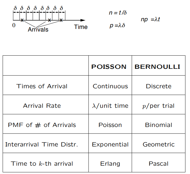
Bernoulli review:如果考虑的是coin tosses,那么我们谈论的是heads和tails;如果我们考虑的是a sequence of trials,那么我们谈论的是sucesses和failures。对于discrete time,我们有time slots,每个time slot我们有independent Bernouli trial。 [mathjax]
- Number of arrivals in \(n\) time slots: 相当于\(n\)个伯努利过程的结果分布满足binomial PMF
- Interarrival times: geometric PMF
- Time to \(k\) arrivals: Pascal PMF 补充
- Memorylessness
The Poisson process is a continuous time version of the Bernoulli process. 银行的前台记录每个time slot(假设是一分钟)内有没有新的顾客进来,当然可以将slot变得更小,比如每秒钟甚至是每万分之一秒。于是我们会问,为啥不直接记录每个新顾客到来的时间呢?
【Poisson point process】定义
- Time homogeneity
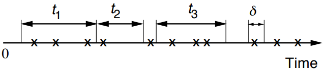
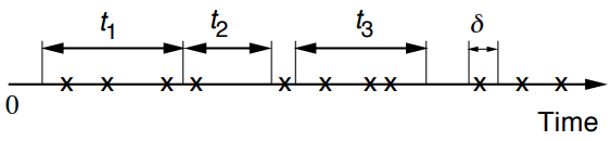
\(P(k, \tau)=\) Prob. of \(k\) arrivals in interval of duration \(\tau\)。如果固定\(\tau\),那么\(\displaystyle\sum_{k} P(k, \tau)=1\)。无论这里的\(\tau\)选在时间轴上的哪里,只要\(\tau\)的长度固定,都是probabilistically same。 - Numbers of arrivals in disjoint time intervals are independent (对应上面的\(t_1\)、\(t_2\)、\(t_3\))。
- Small interval probabilities
For VERY small \(\delta\) : (下面的等式右边严格来说要加上\(o\left(\delta^{2}\right)\),只是在\(\lambda\)很小的情况下这一项可以被忽略)$$ P(k, \delta) \approx \begin{cases}1-\lambda \delta, & \text { if } k=0 \\ \lambda \delta, & \text { if } k=1 \\ 0, & \text { if } k>1\end{cases} $$其中\(\lambda\)为【arrival rate】,expected number of arrivals per unit time,所以我们也将其称作the intensity of this process。更严格的说法是$$\lim _{\delta \rightarrow 0}\frac { P(1, \delta) }{ \delta } =\lambda$$或者等价地表示为$$\lim _{\delta \rightarrow 0}P(1,\delta )=\lim _{\delta \rightarrow 0} \lambda\delta =\lim _{n \rightarrow \infty} \lambda \frac { 1 }{ n }$$这里的\( 1 \)表示的是单位时间,如果我们想研究\(\tau\)时间内的情况而不是单位时间,那么\(\delta = \tau/n\)或者说\( \lambda\tau = np\)。
A visual depiction of a Poisson point process starting from 0 , in which increments occur continuously and independently at rate \(\lambda\).

泊松分布成立的条件:
- counts are of rare events
- all events are independent
- average rate does not change over the period of interest
In physics, these conditions normally occur when we are dealing with counting – especially radioactive decay, or photon counting using a Geiger tube.
【Poisson limit theorem】(泊松极限定理),也是泊松分布的推导。假设某件事情单位时间内发生的次数为\(\lambda\),其实也就是期望,那么将这个单位时间平均分为\( n\)份,那么每份时间内该事件发生的次数\(p=\lambda/n\),当\(n\)趋于无穷大,也就是在单位时间内进行无数次的伯努利实验。那么单位时间内,发生次数为\(k\)的概率为
注:Historically, \(\left(\begin{array}{l}n \\ k\end{array}\right) p^{k}(1-p)^{n-k} \approx \displaystyle\frac{e^{-n p}(n p)^{k}}{k !}\) people approximated the binomial distribution by this for \(n \geqslant 50\) and \(n p \leqslant 5\). Due to modern calculators and computers, this is not used as much.
PMF of Number of Arrivals \(N\)
- Finely discretize \([0, t]\) : approximately Bernoulli
- \(N_{t}\) (of discrete approximation): binomial
- Taking \(\delta \rightarrow 0\) (or \(n \rightarrow \infty\) ) gives:$$ P(k, \tau)=\frac{(\lambda \tau)^{k} e^{-\lambda \tau}}{k !}, \quad k=0,1, \ldots $$再次强调如果固定\(\tau\),那么\(\displaystyle\sum_{k} P(k, \tau)=1\)。
- \(\mathbf{E}\left[N_{t}\right]=\lambda t, \quad \operatorname{var}\left(N_{t}\right)=np(1-p)=\lambda t\)
注:这里用\(t\),而不是\(\tau\),二者是一样的。
泊松分布和指数分布:
- 泊松分布描述一段时间内,事件发生次数的概率分布(已知单位时间内发生的次数)。量纲:次/时间,类似傅里叶变换的频域。PMF(单位时间内)为\(P(X=k)=\displaystyle\frac{e^{-\lambda} \lambda^{k}}{k !}\)。数学期望为\(\lambda\)。
- 指数分布描述的是泊松过程中,相邻两次事件发生的时间间隔的概率分布。量纲:时间,类似傅里叶变换的时域。PDF为\(f(x ; \lambda)= \begin{cases}\lambda e^{-\lambda x} & x \geq 0 \\ 0 & x<0\end{cases}\)。数学期望为\( 1/\lambda \)。
- 例子:超市收银台,平均每分钟有两名顾客结账通过。
以泊松分布计算一分钟内没有顾客通过收银台的概率$$ \begin{aligned} &E(x)=2=\lambda \\ &P(x=0)=\frac{\lambda^{x}}{x !} e^{-\lambda}=\frac{2^{0}}{0 !} e^{-2}=\frac{1}{e^{2}} \end{aligned} $$以指数分布计算,一分钟内没有顾客通过收银台的概率$$ \begin{aligned} &E(t)=\frac{1}{2}=\frac{1}{\lambda} \quad \lambda=2 \\ &P(t>1)=\int_{1}^{+\infty} \lambda e^{-\lambda t} d t=-\left.e^{-2 t}\right|_{1} ^{+\infty}=\frac{1}{e^{2}} \end{aligned} $$
泊松分布与正态分布:
实例:日常生活中,大量事件是有固定频率的(严格来说不太对),比如
- 某医院平均每小时出生3个婴儿
- 某公司平均每10分钟接到1个电话
- 某超市平均每天销售4包xx牌奶粉
- 某网站平均每分钟有2次访问
当我们把时间限定在某个特定小一点的时间段,那么可以认为事件在单位时间内发生的概率/频率是固定的。它们的特点就是,我们可以预估这些事件的总数(单位时间或者说某一段时间内发生的次数,其实也就是期望,但是\(n \)很大,\( p\)很小),但是没法知道具体的发生时间。已知平均每小时出生\(3 \)个婴儿,请问下一个小时/三个小时,出生\(0 \)个婴儿的概率是多少?不记得点这里。
You get email according to a Poisson process at a rate of \(\lambda=5\) messages per hour. You check your email every thirty minutes. Prob(no new messages) ? Prob(one new messages) ?
注:Fix your time slot at 下午一点到两点。那么arrival rate或者说时间发生的频率是固定的,我们可以将其看作泊松过程。下面解法的第一步就是求出我们要研究的时间范围(slot)对应的arrival times,这样就简化了问题。下面的\(P(0,1 / 2)\)中的\( 1/2\)表示的是我们现在研究的time slot范围是给出的采样间隔的\( 1/2\)。$$ \begin{aligned} &\lambda t=5 \cdot \frac{1}{2}=2.5 \\ &P(0,1 / 2)=\frac{(\lambda t)^{0}}{0 !} e^{-\lambda t}=e^{-2.5}=0.08 \\ &P(1,1 / 2)=0.20 \end{aligned} $$
If you have a very, very weak light source that's shooting out photons, just one at a time, the times at which these photons will go out is well modeled again by a Poisson process. Or if you have a radioactive material where one atom at a time changes at random times. So it's a very slow radioactive decay. The time at which these alpha particles, or whatever we get emitted, again is going to be described by a Poisson process. So if you have arrivals, or emissions, that happen at completely random times, and once in a while you get an arrival or an event, then the Poisson process is a very good model for these events.
Interarrival Times
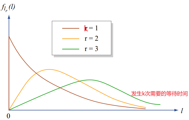
- \(Y_{k}\) time of \(k\) th arrival
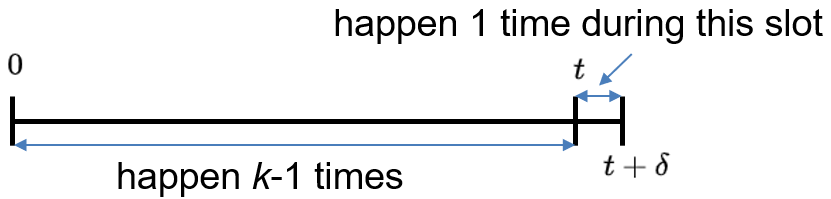
- 【Erlang distribution】$$ f_{Y_{k}}(y)=\frac{\lambda^{k} y^{k-1} e^{-\lambda y}}{(k-1) !}, \quad y \geq 0 $$\( f_{Y_{k}}(t) \delta= P(t \leqslant Y_{k} \leqslant t+\delta )=P(k-1 \,\text{arrivals in} \,[0, t])\cdot\lambda\delta = \displaystyle\frac{(\lambda t)^{k-1}}{(k-1) !} e^{-\lambda t} \cdot \lambda\delta\)
等式两边同时去掉\(\delta\)即得到最终结果。 - Time of first arrival \((k=1)\) : exponential: \(\quad f_{Y_{1}}(y)=\lambda e^{-\lambda y}, \quad y \geq 0\)
- Memoryless property: The time to the next arrival is independent of the past
注:Time of the first arrival in 伯努利过程服从几何分布(分立的),和上面的指数分布(连续的)形状很像,指数分布实际上也是discrete version of 指数分布。 - 指数分布和Erlang distribution是同一类东西:连续分布,表示独立随机事件发生的时间间隔。相比于指数分布,爱尔朗分布能更好地对现实数据进行拟合(更适用于多个串行过程,或无记忆性假设不显著的情况下)。
- 具有\(k\)-Erlang distribution的随机变量和可以看作具有同一指数分布的独立的\(k\)个随机变量之和。
- \(k\)-Erlang distribution在排队模型中得到广泛应用。比如假定顾客在到达窗口排队必须通过一个关口,这个关口由\(k\)层构成,通过每层的时间服从参数为\(\lambda\)的指数分布,那么顾客通过整个关卡到达窗口排队的时间就是Erlang distribution。
- 如果你想simulate泊松过程,你有两种选择:
- break time into tiny, tiny slots. And for every tiny slot, use your random number generator to decide whether there was an arrival or not. To get it very accurate, you would have to use tiny, tiny slots. So that would be a lot of computation.
- The more clever way of simulating the Poisson process is you use your random number generator to generate a sample from an exponential distribution and call that your first arrival time. Then go back to the random number generator, generate another independent sample, again from the same exponential distribution. That's the time between the first and the second arrival, and you keep going that way.
- 参考资料:排队论中的常见分布:泊松分布、指数分布与爱尔朗分布
Bernoulli/Poisson Relation
Merging Poisson Processes
- Sum of independent Poisson random variables is Poisson.
比如假设你每小时能钓上0.4条鱼,假设你总共钓鱼五小时,前两个小时钓到的鱼的数量\(N_{[0,2]}\)满足泊松分布(mean为0.8条鱼),后三个小时钓到的鱼的数量\(N_{[2,3]}\)也满足泊松分布(mean为1.2条鱼),那么这五个小时钓上的鱼的数量\(N_{[0,5]}\)也满足泊松分布(mean为2条鱼)。这说明相同arrival rate的两个具有泊松分布的随机变量之和,即新得到的随机变量也满足泊松分布(arrival rate仍然不变)。 - Merging of independent Poisson processes is Poisson
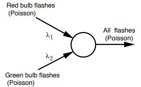
- 红—亮,绿—亮,概率为\(\lambda_{1} \delta \lambda_{2} \delta\)
- 红—亮,绿—灭,概率为\(\lambda_{1} \delta\left(1-\lambda_{2} \delta\right)\),或者\(\lambda_{1} \delta\)。
- 红—灭,绿—亮,概率为\(\left(1-\lambda_{1} \delta\right) \lambda_{2}\delta \),或者\(\lambda_{2}\delta\)。
- 红—灭,绿—灭,概率为\(\left(1-\lambda_{1} \delta\right) \left(1-\lambda_{2} \delta\right)\)或者\(1-\lambda_{1} \delta-\lambda_{2} \delta\)
- 因此,考虑all flashes,see arrival with all probability约为\( (\lambda_{1}+\lambda_{2}) \delta\)。
- What is the probability that the next arrival comes from the first process(red)?约为\(\displaystyle\frac{\lambda_{1}}{\lambda_{1}+\lambda_{2}}\)
Poissonian Process in Physics/Measurement
(1) Zero-temperature Franck–Condon factors$$ F_{n}^{0}=\left|\int \psi_{0}^{*} \psi_{n} \mathrm{~d} Q\right|^{2}=\frac{\mathrm{e}^{-S} S^{n}}{n !} $$The interpretation of this equation is that the number of excited vibrational quanta in the transition is Poisson distributed around an average of \(S\). 参考资料[Mathijs de Jong-PCCP]
(2) Radioactive source
Radioactive source emitting 1000 photons/s, long half life, 4 s measurement, detector \(0.1 \%\) sensitivity. 求probability of detecting at least 2 photons in a 4 s measurement?
对常见的一级反应动力学的放射性物质来说,半衰期对应的时间其实就是\(\displaystyle\frac{\ln 2}{\lambda}\),或者说对应于我们荧光粉单指数衰减寿命的\(\ln 2\)倍。我们荧光粉算寿命是衰减到初始状态的\(1/e\),而不是半衰期计算用的\(1/2\)。题目里的long half life其实是和4 s对比的,意在表面在4 s这个时间尺度内我们可以认为放射源单位时间放出的光子数是不变的。
期望\(\mu=1000 \displaystyle\frac{1}{\mathrm{s}} \cdot 4 \mathrm{s} \cdot 0.001=4\),于是所求概率为
$$P({n} \geq 2, \mu=4)=1-(P({n}=0, \mu=4)+P({n}=1, \mu=4))=1-5e^{-4} \approx 0.91$$
(3) Astronomical sources produce photons
The vast majority of astronomical sources produce photons via random processes distributed over vast scales. Therefore, when these photons arrive at the Earth, they are randomly spaced, as illustrated in the figure a. The number of photons counted in a short time interval will vary, even if the long-term mean number of photons is constant. This variation is known as 【shot noise】. It represents the irreducible minimum level of noise present in an astronomical observation.
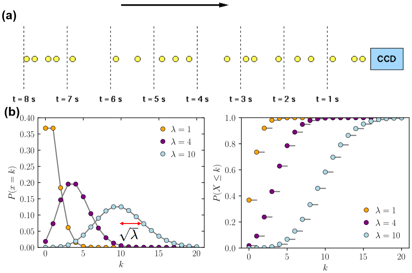
图a:Photons from a faint, non-variable astronomical source incident on a CCD detector. Because the signal is low in this example, it is easy to see that there is a substantial variation in the number of photons detected in each 1 s time interval.
图b:\(\lambda\)表示的是the mean of the distribution,对应的标准差为\(\sqrt{\lambda}\),横轴表示的是每秒探测到的光子数\(k\),纵轴表示对应的概率\(P(x=k)\)。
If one plots a histogram of the number of photons arriving in each time interval, the resulting distribution is known as a Poisson distribution, as shown in figure 116. Poisson statistics are applicable when counting independent, random events which occur, when measured over a long period of time, at a constant rate. The Poisson distribution is therefore applicable to the counting of photons from astronomical sources, the counting of photons from the sky, or the production of thermally-generated electrons in a semi-conductor (i.e. dark current).
对于\(\mu = 10\),the fractional error\(\mu/\sqrt{\lambda}=0.316\),如果\(\mu = 100\),那么the fractional error变为0.10。This shows that as more photons are counted, the noise becomes a smaller fraction of the signal, i.e. the SNR (signal-to-noise ratio) improves. 参考photon statistics-Vik Dhillon
(4) Medical Radiography System's Image Quality
参考[Storage Phosphors for Medical Imaging-Materials-2011]
x
参考资料:
(1) Poissonian Distributions in Physics: Counting Electrons and Photons-2021
(2) Poisson distribution and application-2008
(3) Photon Counting Statistics and the Poisson Distribution
Markov Chains
Weak Law of Large Numbers
Central Limit Theorem
Bayesian Statistical Inference
Classical Statistical Inference
经典分布中文
高斯分布
\(f(x)=\frac{1}{\sigma \sqrt{2 \pi}} e^{-\frac{(x-\mu)^{2}}{2 \sigma^{2}}}\) 高斯分布最早的提出者是棣莫弗,但是高斯毕竟数学王子,正如李永乐说的,人类历史上的三大数学家是阿基米德、牛顿、高斯,如果是四大数学家,那么就加上欧拉。其实这个棣莫弗也是一位著名的数学家,他首次将复数和三角函数联系在一起,他最著名的贡献是棣莫弗公式,对任意复数\(x\)和整数\(n\),存在如下关系: \((\cos (x)+i \sin (x))^{n}=\cos (n x)+i \sin (n x)\) 这其实就是欧拉公式的一种特例。
小知识
Error propagation
补充
参考资料:
(1) Error propagation—UCL