FFT

FFT是上个世纪发明的在伟大的算法之一，无线通讯、GPS等等都依赖与FFT。

对于一个\( d\)次多项式，我们有两种unique 【polynomial representations】$$ P(x)=p_{0}+p_{1} x+p_{2} x^{2}+\cdots+p_{d} x^{d} $$(1)【Coefficient Representation】，即用每一个不同次数项的系数组\(\left[p_{0}, p_{1}, \ldots, p_{d}\right]\)来描述。

(2)【Value Representation】
选取\((d+1)\) points，同样可以唯一地确定这个多项式。比如选取这些点$$\left\{\left(x_{0}, P\left(x_{0}\right)\right),\left(x_{1}, P\left(x_{1}\right)\right), \ldots,\left(x_{d}, P\left(x_{d}\right)\right)\right\}$$然后写成矩阵乘法的形式为$$ \left[\begin{array}{c} P\left(x_{0}\right) \\ P\left(x_{1}\right) \\ \vdots \\ P\left(x_{d}\right) \end{array}\right]=\left[\begin{array}{ccccc} 1 & x_{0} & x_{0}^{2} & \cdots & x_{0}^{d} \\ 1 & x_{1} & x_{1}^{2} & \cdots & x_{1}^{d} \\ \vdots & \vdots & \vdots & \ddots & \vdots \\ 1 & x_{d} & x_{d}^{2} & \cdots & x_{d}^{d} \end{array}\right]\left[\begin{array}{c} p_{0} \\ p_{1} \\ \vdots \\ p_{d} \end{array}\right] $$其中的系数矩阵\(M\) is invertible for unique \(x_{0}, x_{1}, \ldots, x_{d}\)，系数矩阵是否可逆可以通过计算行列式来判定，显然对于可逆矩阵，必然有唯一解，即对应于唯一的多项式\(P(x)\)。

 

两种表示方法的算法复杂度对比

采用这种Value Representation的好处是多项式的乘法变得更简单。下面举例说明：对于$$ A(x)=x^{2}+2 x+1 \quad B(x)=x^{2}-2 x+1 \quad C(x)=A(x) \cdot B(x) $$的计算，如果我们在\(  A(x)\)和\(B(x)\)上各取\(5\)个点，注意取点的时候\( x\)的位置要一致。然后将对应位置的函数值相乘，即\begin{aligned} &\,{[(-2,1),(-1,0),(0,1),(1,4),(2,9)]} \\ &\frac{[(-2,9),(-1,4),(0,1),(1,0),(2,1)]}{[(-2,9),(-1,0),(0,1),(1,0),(2,9)]} \end{aligned}于是我们可以用\([(-2,9),(-1,0),(0,1),(1,0),(2,9)]\)这\(5\)个点来表示\(4\)次多项式\( C(x)\)。Multiplication in value representation is only \(O(d)\) ! 对比之前的Coefficient Representation，由于\(A(x)\)中每一项都要和\(B(x)\)中的每一项相乘，所以算法复杂度为\(O\left(d^{2}\right)\)。

 

多项式乘法的变换流程

(1) Coeff \(\Rightarrow\) Value

对于\(P(x)=p_{0}+p_{1} x+p_{2} x^{2}+\cdots+p_{d} x^{d}\)，我们想要Evaluate at \(n \geq d+1\) points，那么要找到\(n\)个点的坐标我们需要进行如下计算，取\(x\)为\(1\)到\(n\)的一系列正整数$$ \begin{gathered} \left(1, p_{0}+p_{1} \cdot 1+p_{2} \cdot 1^{2}+\cdots+p_{d} \cdot 1^{d}\right) \\ \left(2, p_{0}+p_{1} \cdot 2+p_{2} \cdot 2^{2}+\cdots+p_{d} \cdot 2^{d}\right) \\ \vdots \\ \left(n, p_{0}+p_{1} \cdot n+p_{2} \cdot n^{2}+\cdots+p_{d} \cdot n^{d}\right) \end{gathered} $$算法复杂度，由于\(n \geq d+1\)因此$$ O(n d) \Leftrightarrow O\left(d^{2}\right) $$下面对其进行简化过程，要利用的性质就是对于\(x^m\)次方的奇偶特性，当幂次项为奇数，那么函数为奇函数，否则为偶函数。对于$$ P(x)=3 x^{5}+2 x^{4}+x^{3}+7 x^{2}+5 x+1 $$我们对称地选取\(n=6\)个点\(\pm x_{1}, \pm x_{2}, \ldots, \pm x_{n / 2}\)，(注意我们按\(1\)到\(n\)的取法的话，函数奇偶性的特点就用不上了)，那么多项式可以改写为$$P(x)=\underbrace{\left(2 x^{4}+7 x^{2}+1\right)}_{P_{e}\left(x^{2}\right)}+ x\underbrace{\left(3 x^{4}+x^{2}+5\right)}_{P_{o}\left(x^{2}\right)}$$更一般的情况，我们可以表示为如下(其中\(i=\{1,2, \ldots, n / 2\}\))$$ \begin{gathered} P(x)=P_{e}\left(x^{2}\right)+x P_{o}\left(x^{2}\right) \\ P\left(x_{i}\right)=P_{e}\left(x_{i}^{2}\right)+x_{i} P_{o}\left(x_{i}^{2}\right) \\ P\left(-x_{i}\right)=P_{e}\left(x_{i}^{2}\right)-x_{i} P_{o}\left(x_{i}^{2}\right) \end{gathered} $$\(P_{e}\left(x^{2}\right)\) and \(P_{o}\left(x^{2}\right)\) have degree \(n / 2-1 !\) 这里有点像机器学习或者线性代数中的降维过程。现在我们只需要Evaluate一半的点(\((n / 2\) points个)函数值，即取\(x\)轴的正半部分，通过这一半的点，我们可计算Evaluate\(P_{e}\left(x^{2}\right)\) and \(P_{o}\left(x^{2}\right)\) each at \(x_{1}^{2}, x_{2}^{2}, \ldots, x_{n / 2}^{2}\)，显然通过这部分的计算结果可以较为容易地推出\(x\)轴的负半部分对应的函数值。

从上面看，我们简化了运算，但是只能简化一次，不能继续简化，因为第一次简化后，我们的计算对象的横坐标不再是正负pair，即我们不能再利用多项式的奇偶特性了。

Points \(\left[\pm x_{1}, \pm x_{2}, \ldots, \pm x_{n / 2}\right]\) are \(\pm\) paired.
Points \(\left[x_{1}^{2}, x_{2}^{2}, \ldots, x_{n / 2}^{2}\right]\) are not \(\pm\) paired.
Recursion breaks! Is it possible to make \(\left[x_{1}^{2}, x_{2}^{2}, \ldots, x_{n / 2}^{2}\right] \pm\) paired?

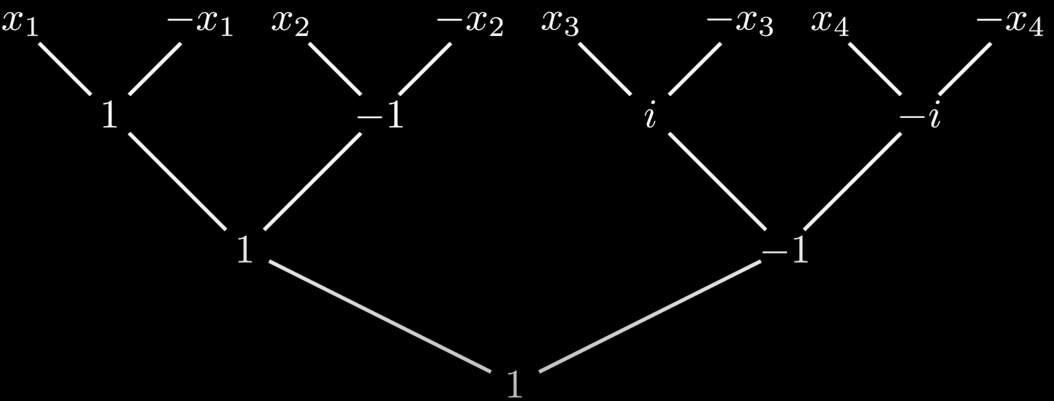
例子：对于\(P(x)=x^{3}+x^{2}-x-1\)，我们需要每次迭代后(即对原来的数据点的横轴取平方)，仍然得到一组点，其横轴坐标的集合也是满足继续迭代的要求(正负pair)。
对于Solution to \(x^{4}=1\)，Points are \(4^{\text {th }}\) roots of unity!业就是说上图中最上层的四个数据分别对应\(x^{4}=1\)的不同根。

进一步得，对于\(P(x)=x^{5}+2 x^{4}-x^{3}+x^{2}+1\)。Need \(n \geq 6\) points \(\rightarrow\) let \(n=8\) (powers of 2 are convenient)
对于更一般的情形，\(P(x)=p_{0}+p_{1} x+p_{2} x^{2}+\cdots+p_{d} x^{d}\)。Need \(n \geq(d+1)\) points, \(n=2^{k}, k \in \mathbb{Z}\). Points are \(8^{\text {th }}\) roots of unity!
这里我们让就对原点而言中心对称的点组成pair，即两个点的连线通过原点。换句话说，就是一个点对应的角度减去另一个店对应的角度，正好等于\( \pi\)，也就是这个圆\(n\)等分的情况下，\(n/2 \)次power of \(\omega \)。$$ \omega^{j+n / 2}=-\omega^{j} \rightarrow\left(\omega^{j}, \omega^{j+n / 2}\right) \text { are } \pm \text { paired } $$

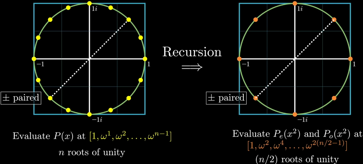
总结一下，注意$$\begin{array}{cc} x_{j}=\omega^{j} & y_{e}[j]=P_{e}\left(\omega^{2 j}\right) \\ -\omega^{j}=\omega^{j+n / 2} & y_{o}[j]=P_{o}\left(\omega^{2 j}\right) \end{array}$$

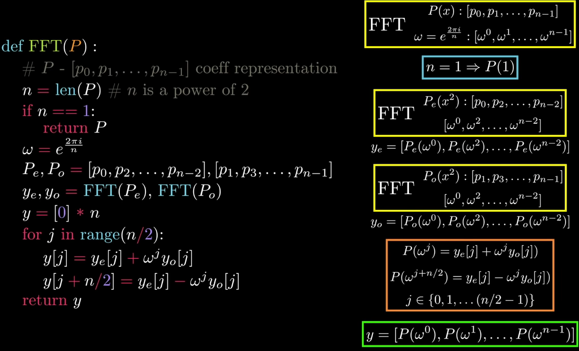
对于多项式\(\bar{P}(x)=p_{0}+p_{1} x+p_{2} x^{2}+\cdots+p_{n-1} x^{n-1}\)，可以写成矩阵乘法，如果令\(x_{k}=\omega^{k}\) where \(\omega=e^{\frac{2 \pi i}{n}}\)，那么就可以得到FFT的形式。$$ \left[\begin{array}{c} P\left(x_{0}\right) \\ P\left(x_{1}\right) \\ P\left(x_{2}\right) \\ \vdots \\ P\left(x_{n-1}\right) \end{array}\right]=\left[\begin{array}{ccccc} 1 & x_{0} & x_{0}^{2} & \cdots & x_{0}^{n-1} \\ 1 & x_{1} & x_{1}^{2} & \cdots & x_{1}^{n-1} \\ 1 & x_{2} & x_{2}^{2} & \cdots & x_{2}^{n-1} \\ \vdots & \vdots & \vdots & \ddots & \vdots \\ 1 & x_{n-1} & x_{n-1}^{2} & \cdots & x_{n-1}^{n-1} \end{array}\right]\left[\begin{array}{c} p_{0} \\ p_{1} \\ p_{2} \\ \vdots \\ p_{n-1} \end{array}\right] $$

FFT和IFFT的对比

FFT：已知基和系数，求函数值，即\(Ax=b\)中，求\(b\)。
\(\operatorname{FFT}\left(\left[p_{0}, p_{1}, \ldots, p_{n-1}\right]\right) \rightarrow\left[P\left(\omega^{0}\right), P\left(\omega^{1}\right), \ldots, P\left(\omega^{n-1}\right)\right]\)，即求解矩阵$$ \left[\begin{array}{c} P\left(\omega^{0}\right) \\ P\left(\omega^{1}\right) \\ P\left(\omega^{2}\right) \\ \vdots \\ P\left(\omega^{n-1}\right) \end{array}\right]=\left[\begin{array}{ccccc} 1 & 1 & 1 & \cdots & 1 \\ 1 & \omega & \omega^{2} & \cdots & \omega^{n-1} \\ 1 & \omega^{2} & \omega^{4} & \cdots & \omega^{2(n-1)} \\ \vdots & \vdots & \vdots & \ddots & \vdots \\ 1 & \omega^{n-1} & \omega^{2(n-1)} & \cdots & \omega^{(n-1)(n-1)} \end{array}\right]\left[\begin{array}{c} p_{0} \\ p_{1} \\ p_{2} \\ \vdots \\ p_{n-1} \end{array}\right] $$其中\(\operatorname{FFT}(<\) coeffs \(>)\) defined \(\omega=e^{\frac{2 \pi i}{n}}\)

---

IFFT：已知基和函数，求系数，即\(Ax=b\)，已知\(x\)。
\(\operatorname{IFFT}\left(\left[P\left(\omega^{0}\right), P\left(\omega^{1}\right), \ldots, P\left(\omega^{n-1}\right)\right]\right) \rightarrow\left[p_{0}, p_{1}, \ldots, p_{n-1}\right]\)，即求解矩阵$$ \left[\begin{array}{c} p_{0} \\ p_{1} \\ p_{2} \\ \vdots \\ p_{n-1} \end{array}\right]=\frac{1}{n}\left[\begin{array}{ccccc} 1 & 1 & 1 & \cdots & 1 \\ 1 & \omega^{-1} & \omega^{-2} & \cdots & \omega^{-(n-1)} \\ 1 & \omega^{-2} & \omega^{-4} & \cdots & \omega^{-2(n-1)} \\ \vdots & \vdots & \vdots & \ddots & \vdots \\ 1 & \omega^{-(n-1)} & \omega^{-2(n-1)} & \cdots & \omega^{-(n-1)(n-1)} \end{array}\right]\left[\begin{array}{c} P\left(\omega^{0}\right) \\ P\left(\omega^{1}\right) \\ P\left(\omega^{2}\right) \\ \vdots \\ P\left(\omega^{n-1}\right) \end{array}\right] $$Every \(\omega\) in DFT matrix is now \(\displaystyle\frac{1}{n} \omega^{-1}\)
注：通过重新定义FFT中的\(\omega \)可以等价地描述其对应的IFFT，即$$ \operatorname{IFFT}(<\text { values }>) \Leftrightarrow \mathrm{FFT}(<\text { values }>) \text { with } \omega=\frac{1}{n} e^{\frac{-2 \pi i}{n}} $$

我的思考：
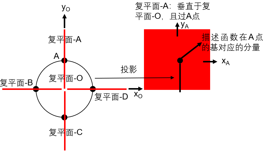
(1) 既然FFT的基在二维复平面上，那么我们可以先画出二维复平面上所有的基对应的点，然后对每个点做对称于该圆且交于该点的平面，其实就是相当于这个点的复平面，那么函数在该点的分量，就可以用该平面上的一个点来描述。

(2) FFT和IFFT矩阵，有的人将提到外面的系数都表示为\(1/\sqrt{n}\)，这样保证两个矩阵的系数的乘积还是\(1/n \)。

(3) FFT和IFFT的内核还是\(Ax=b\)，将矩阵\( A\)作用在\(x\)上能得到\(b\)，和将矩阵\(A^{-1}\)作用在\(b\)上能得到\(  x\)其实就是正变换和逆变换。

(4) 既然可以用\(Ax=b\)来描述FFT或者IFFT，那么显然也可以就FFT matrix或者IFFT matrix的特征值与特征向量。当然了，连续傅里叶变换，其实可以看作上面的极限情况，其变换过程，也有对应的特征值和特征向量。最特殊的情况，比如对高斯函数做傅里叶变换，得到的还是高斯函数，那么显然高斯函数就是特征向量。

(5) 我们上面从多项式进入到FFT，易知全体多项式就构成了一个线性空间，显然多项式\(P(x)\)和\(Q(x)\)的加和还在这个线性空间中，多项式\(P(x)\)乘以一个常数得到的还是一个多项式，显然满足线性空间的八条公理。同样地，矩阵描述的也是一种线性空间，

参考资料：
(1) The Fast Fourier Transform (FFT): Most Ingenious Algorithm Ever?-油管

 

Z变换

希尔伯特变换

解析信号

Much of digital signal processing requires working with negative frequencies. Negative frequencies in practice do not mean anything and introducing such frequencies in digital signal processing analysis may be troublesome. It is easy to convert a signal that contains negative frequencies into one that does not. A converter that removes negative frequencies from an analytical signal is called a 【Hilbert transform】.

【解析信号】(analytic signal)：在数学和信号处理中，解析信号是没有负频率分量的复值函数。解析信号的实部和虚部是由希尔伯特变换相关联的实值函数。The analytic representation of a real-valued function is an analytic signal, comprising the original function and its Hilbert transform.

表示成解析信号的好处：This representation facilitates many mathematical manipulations. The basic idea is that the negative frequency components of the Fourier transform (or spectrum) of a real-valued function are superfluous (多余的), due to the Hermitian symmetry of such a spectrum. These negative frequency components can be discarded with no loss of information, provided one is willing to deal with a complex-valued function instead. That makes certain attributes of the function more accessible and facilitates the derivation of modulation and demodulation techniques, such as single-sideband.

解析信号到实际信号：As long as the manipulated function has no negative frequency components (that is, it is still analytic), the conversion from complex back to real is just a matter of discarding the imaginary part. The analytic representation is a generalization of the phasor (向量，矢量) concept: while the phasor is restricted to time-invariant amplitude, phase, and frequency, the analytic signal allows for time-variable parameters.

如果\(s(t)\)是一个实数函数，其傅里叶变换为\(S(f)\)，则\(S(f)\)对于\(f=0\)轴具有Hermitian symmetry，即\(S(-f)=S(f)^*\)。定义函数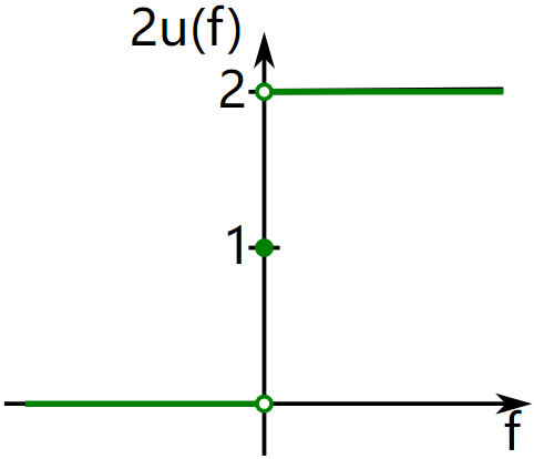$$ \begin{aligned} S_{\mathrm{a}}(f) & \triangleq \begin{cases}2 S(f), & \text { for } f>0, \\ S(f), & \text { for } f=0, \\ 0, & \text { for } f<0\end{cases} \\ & =\underbrace{2 \mathrm{u}(f)}_{1+\operatorname{sgn}(f)} S(f)=S(f)+\operatorname{sgn}(f) S(f) \end{aligned} $$其中\(u(f)\)为Heaviside step function，\(\operatorname{sgn}(f)\)为sign function。那么\(S_{\mathrm{a}}(f)\)只含有\(S(f)\)非负频率的分量。显然，由于\(S(f)\)的Hermitian symmetry特点，我们也可以通过\(S_{\mathrm{a}}(f)\)来表示\(S(f)\)，二者的转换是reversible的。实数函数\(s(t)\)的解析信号，就是\(S_{\mathrm{a}}(f)\)的傅里叶逆变换。
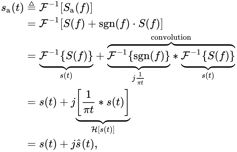其中\(\hat{s}(t) \triangleq \mathcal{H}[s(t)]\)为\(s(t)\)的希尔伯特变换；\(*\)是binary convolution operator；\(j\)是虚部单位。

Noting that \(s(t)=s(t) * \delta(t)\), this can also be expressed as a filtering operation that directly removes negative frequency components:$$ s_{\mathrm{a}}(t)=s(t) * \underbrace{\left[\delta(t)+j \frac{1}{\pi t}\right]}_{\mathcal{F}^{-1}\{2 u(f)\}} $$正如我们在之前傅里叶变换的笔记中谈到的那样，时域的卷积对应于频域的乘法，即上式频域的写法为\(S_{\mathrm{a}}(f)=S(f) 2 \mathrm{u}(f)\)。

负频率分量：由\(s_{\mathrm{a}}(t)=s(t)+j \hat{s}(t)\)，易知\(s(t)=\operatorname{Re}\left[s_{\mathrm{a}}(t)\right]\)，即恢复负频率分量可以通过丢掉解析信号虚部的方法来实现。同样对于\(s_{\mathrm{a}}^*(t)\) comprises only the negative frequency components. And therefore \(s(t)=\operatorname{Re}\left[s_{\mathrm{a}}^*(t)\right]\) restores the suppressed positive frequency components. Another viewpoint is that the imaginary component in either case is a term that subtracts frequency components from \( s(t)\). The \(\operatorname{Re}\) operator removes the subtraction, giving the appearance of adding new components.

Analytic signal的例子：

例子-1，\(s(t)=\cos (\omega t)\), where \(\omega>0\)
\(s(t)\)的希尔伯特变换\(\hat{s}(t)=\displaystyle\frac{1}{\pi t} * s(t)\)，写成对应频域的形式，右侧可以表示为\( \mathcal{F}(\displaystyle\frac{1}{\pi t})\mathcal{F}(s(t))=-i  \cdot \operatorname{sgn}(f)S(f)\)，即对\(S(f)\)正频率的部分乘以\(-i\)，对负频率的部分乘以\( i\)。假设某个正频率\(f\)对应的分量表示为\(a+ib\)，那么乘以\(- i\)之后就变成了\(b-ia\)，即顺时针旋转了90度相位。总之无论是从相位移动上去理解还是直接算傅里叶变换，我们都将得到如下结果：$$ \begin{aligned} \hat{s}(t) & =\cos \left(\omega t-\frac{\pi}{2}\right)=\sin (\omega t) \\ s_{\mathrm{a}}(t) & =s(t)+j \hat{s}(t)=\cos (\omega t)+j \sin (\omega t)=e^{j \omega t} \end{aligned} $$回忆一下由欧拉公式我们有\(\cos (\omega t)=\frac{1}{2}\left(e^{j \omega t}+e^{j(-\omega) t}\right)\)，丢弃其中的负频率，然后让正频率翻倍，即得到上面的结果。

例子-2，Here we use Euler's formula to identify and discard the negative frequency.$$ s(t)=\cos (\omega t+\theta)=\frac{1}{2}\left(e^{j(\omega t+\theta)}+e^{-j(\omega t+\theta)}\right) $$Then:$$ s_{\mathrm{a}}(t)= \begin{cases}e^{j(\omega t+\theta)}=e^{j|\omega| t} \cdot e^{j \theta}, & \text { if } \omega>0 \\ e^{-j(\omega t+\theta)}=e^{j|\omega| t} \cdot e^{-j \theta}, & \text { if } \omega<0\end{cases} $$

性质：待补充

希尔伯特变换

Relationship with the Fourier transform: \( \mathcal{F}(\mathrm{H}(u))(\omega)=-i \operatorname{sgn}(\omega) \cdot \mathcal{F}(u)(\omega)\)其中$$ -i \operatorname{sgn}(\omega)=\left\{\begin{array}{cc} i=e^{+\frac{i \pi}{2}}, & \text { for } \omega<0 \\ 0, & \text { for } \omega=0 \\ -i=e^{-\frac{i \pi}{2}}, & \text { for } \omega>0 \end{array}\right. $$

为什么需要希尔伯特变换：

参考资料：

联系希尔伯特一起写

1

2

3

4

希尔伯特变换和瞬时频率问题--连载（二）

K-K关系

 

参考资料：
(1) 希尔伯特变换将信号表示为复解析信号的物理意义是什么？—知乎